


This study aimed to explain a joint statistical procedure (two-part models and Cholesky decomposition) to incorporate second-order uncertainty from covariate adjusted mean utility functions in probabilistic cost-effectiveness models. First, two-part models were applied to obtain parameters for the utility function. Second, a new set of correlated parameters for each simulation was obtained by Cholesky decomposition. The procedure was applied to EuroQol5D-5L in the Spanish Health Survey (21,007 adults). An example for the first simulation showed that 71% of men aged 60 years, high social status and normal weight were in perfect health, and in those not in perfect health, the expected utility was 0.8474 (= 1 − 0.1526). Therefore, their estimated mean utility value was 0.9559. Mean utility values in the interval (− ∞1] were calculated and their associated uncertainty incorporated in the cost-effectiveness models, based on the uncertainty related to correlated parameters in the utilities function.
El objetivo de este estudio fue explicar el procedimiento estadístico conjunto (modelos en dos etapas y descomposición de Cholesky) para incorporar la incertidumbre de segundo orden asociada a la función de utilidad media ajustada por variables en los modelos probabilísticos de coste-efectividad. Primero se aplicaron los modelos en dos etapas para obtener los parámetros de la función de utilidad. Segundo, para cada simulación, se obtuvo un nuevo conjunto de parámetros correlacionados utilizando la descomposición de Cholesky. El procedimiento se aplicó al cuestionario EuroQol5D-5L de la Encuesta Nacional de Salud en España (21.007 adultos). El ejemplo de una primera simulación mostró que el 71% de los hombres de 60 años, con clase social alta y peso normal tenían una salud perfecta, y en aquellos que no tenían una salud perfecta la utilidad esperada fue de 0,8474 (= 1 − 0,1526). Por lo tanto, su utilidad media estimada fue de 0,9559. Se calcularon utilidades medias con valores comprendidos en el intervalo (-∞1] y se incorporó la incertidumbre asociada a ellos en los modelos de coste-efectividad, basándose en la incertidumbre correspondiente a los parámetros correlacionados de la función de utilidad.
Quality-adjusted life year is the most frequently used instrument to measure health and thus estimate effectiveness in economic evaluation (EE).1 Although it is defined as the integral of the health utility function differential of time, usually the calculation is simplified with use of the corresponding mean health utility multiplied by survival time in that health state.1 In addition, in decision modeling based EE, it is assumed that individuals with the same characteristics will also have the same mean utility value during the whole period of time in a specific health state (there is no first-order uncertainty), while Monte Carlo simulation method is used, in general, to propagate uncertainty around the input parameters (“second-order uncertainty”) to the main outcomes (e.g., incremental cost-effectiveness ratio). In fact, when a regression model is used to estimate mean utility values, utilities’ uncertainty can be defined in terms of uncertainty (and correlation) in the regression model coefficients.2
Several researchers have attempted to identify the best statistical approach to modeling utility data dealing with the upper bound of 1 when individual data are available.3–5 Models such as Tobit, Censored Least Absolute Deviations or Ordinary Least Square are not considered appropriate because utilities by definition are ranged (-∞1] 3,5,6 As an alternative method, two-part models have been proposed.5,7 Two-part models ensure that estimated values will never adopt values higher than 1, while also allowing for negative mean utility values.5,7
Utility functions based on two-part models are used to yield a mean value for each Monte Carlo simulation. In those simulating systems with multiple correlated parameters, Cholesky decomposition is used in order to integrate results of two-part models in probabilistic cost-effectiveness models.1 This study aimed to explain and apply a statistical procedure based on two-part models and the related variance-covariance matrix Cholesky decomposition to incorporate second-order uncertainty for covariate adjusted mean utility functions in probabilistic cost-effectiveness models.
It was not necessary to obtain the approval of the ethics committee since the data used in this study come from the Spanish Statistical Office webpage, where the data are publicly available and the participants included are anonymized.
Method expositionThe two part model5,7 is based on the decomposition of the mean utility value u(x) as follows:

assuming px is the probability of being in perfect health and wx corresponds to the disutility value for those not in perfect health ux<1 and x is a set of covariates. Though, the set of covariates can be different for each model we will assume it is the same in order to simplify.
When individually reported utility data are available, the steps to fit a two-part model have as follows: first, a logistic regression model is applied to estimate the probability px of being in perfect health i.e.ux=1.

Second, the individuals not in perfect health are sub-selected and a generalized linear model (with log link if necessary) is applied to the disutilities i.e.1−ux.

This approach ensures that our final estimate of mean utility does not fall beyond 1 and, at the same time, allows ux to be negative (see online Appendix 1).
When the regression analyses are defined, both estimated coefficient vectors Beta1,Beta2 and their correspondent variance-covariance matrixes V1,V2 should be obtained, where Beta1 and Beta2 are the vectors of coefficients estimated for regression in step 1 and 2 respectively and V1 and V2 their respective variance-covariance matrixes. According to the methodology described in detail by Briggs et al.,1 the Cholesky decomposition of the variance-covariance matrixes V1,V2 will yield the correspondent lower triangular matrixes (T1,T2):

where Ti' is Ti transposed for i=1,2.
Based on the estimated coefficients vector Beta1,Beta2 and obtained triangular matrixes (T1,T2), together with vectors of randomly generated values that each follows a standard Normal distribution Z∼N0,1Z1,Z2, new regression parameters Beta1*,Beta2* were calculated as follows:


That permits, estimating random mean utility values depending on the selected covariates. Confidence intervals would also be estimated based on Monte Carlo simulations.
Practical applicationThis statistical procedure was applied to the Spanish Health Survey performed in 2012 by the Spanish Ministry of Health, Social Services and Equality.8 This survey included 21,007 adults, where 63% of those that responded to the EuroQol 5D-5L questionnaire9 were in perfect health (see online Appendix 2) and the mean utility value was 0.91.
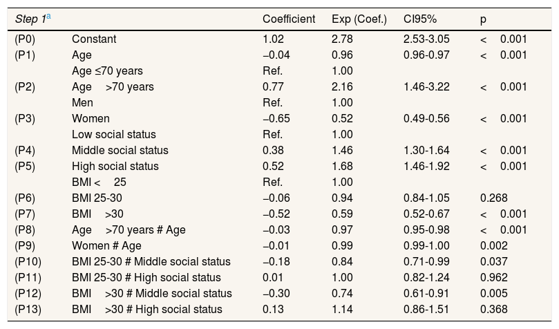
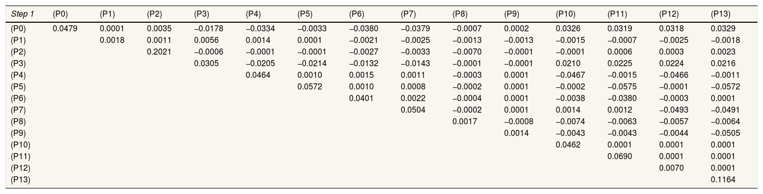
Table 1 shows the coefficients Beta1,Beta2 of the two-part predictive model used, which included covariates of age, sex, social status and body mass index (BMI). Generalized linear model with distribution Poisson and link logarithmic was applied in the second step. The Cholesky decomposition of the variance-covariance matrix in the first T1 and second step T2 are shown in Table 2.
Multivariate regression coefficients in two steps to predict the mean utilities by age, sex, social status and body mass index..
| Step 1a | Coefficient | Exp (Coef.) | CI95% | p | |
|---|---|---|---|---|---|
| (P0) | Constant | 1.02 | 2.78 | 2.53-3.05 | <0.001 |
| (P1) | Age | −0.04 | 0.96 | 0.96-0.97 | <0.001 |
| Age ≤70 years | Ref. | 1.00 | |||
| (P2) | Age>70 years | 0.77 | 2.16 | 1.46-3.22 | <0.001 |
| Men | Ref. | 1.00 | |||
| (P3) | Women | −0.65 | 0.52 | 0.49-0.56 | <0.001 |
| Low social status | Ref. | 1.00 | |||
| (P4) | Middle social status | 0.38 | 1.46 | 1.30-1.64 | <0.001 |
| (P5) | High social status | 0.52 | 1.68 | 1.46-1.92 | <0.001 |
| BMI <25 | Ref. | 1.00 | |||
| (P6) | BMI 25-30 | −0.06 | 0.94 | 0.84-1.05 | 0.268 |
| (P7) | BMI>30 | −0.52 | 0.59 | 0.52-0.67 | <0.001 |
| (P8) | Age>70 years # Age | −0.03 | 0.97 | 0.95-0.98 | <0.001 |
| (P9) | Women # Age | −0.01 | 0.99 | 0.99-1.00 | 0.002 |
| (P10) | BMI 25-30 # Middle social status | −0.18 | 0.84 | 0.71-0.99 | 0.037 |
| (P11) | BMI 25-30 # High social status | 0.01 | 1.00 | 0.82-1.24 | 0.962 |
| (P12) | BMI>30 # Middle social status | −0.30 | 0.74 | 0.61-0.91 | 0.005 |
| (P13) | BMI>30 # High social status | 0.13 | 1.14 | 0.86-1.51 | 0.368 |
| Step 2b | |||||
| (P0) | Constant | −1.74 | 0.18 | 0.16-0.19 | <0.001 |
| (P1) | Age | 0.01 | 1.01 | 1.01-1.01 | <0.001 |
| Age ≤70 years | Ref. | 1.00 | |||
| (P2) | Age> 70 years | −0.53 | 0.60 | 0.50-0.69 | <0.001 |
| Men | Ref. | 1.00 | |||
| (P3) | Women | 0.08 | 1.09 | 1.03-1.15 | 0.004 |
| Low social status | Ref. | 1.00 | |||
| (P4) | Middle social status | −0.03 | 0.97 | 0.89-1.06 | 0.483 |
| (P5) | High social status | −0.18 | 0.84 | 0.76-0.92 | <0.001 |
| BMI <25 | Ref. | 1.00 | |||
| (P6) | BMI 25-30 | −0.01 | 0.99 | 0.92-1.06 | 0.789 |
| (P7) | BMI>30 | 0.21 | 1.23 | 1.15-1.33 | <0.001 |
| (P8) | Age>70 years # Age | 0.02 | 1.02 | 1.02-1.03 | <0.001 |
| (P9) | Women # Age | 0.00 | 1.00 | 1.00-1.01 | <0.001 |
| (P10) | BMI 25-30 # Middle social status | −0.06 | 0.95 | 0.84-1.06 | 0.326 |
| (P11) | BMI 25-30 # High social status | 0.11 | 1.11 | 0.97-1.28 | 0.136 |
| (P12) | BMI>30 # Middle social status | −0.03 | 0.97 | 0.85-1.10 | 0.629 |
| (P13) | BMI>30 # High social status | 0.17 | 1.19 | 0.99-1.43 | 0.065 |
CI95%: confidence interval of 95%; BMI: body mass index.
Triangular matrixes obtained by Cholesky decomposition of the variance-covariance matrix of each multivariate regression.
| Step 1 | (P0) | (P1) | (P2) | (P3) | (P4) | (P5) | (P6) | (P7) | (P8) | (P9) | (P10) | (P11) | (P12) | (P13) |
|---|---|---|---|---|---|---|---|---|---|---|---|---|---|---|
| (P0) | 0.0479 | 0.0001 | 0.0035 | −0.0178 | −0.0334 | −0.0033 | −0.0380 | −0.0379 | −0.0007 | 0.0002 | 0.0326 | 0.0319 | 0.0318 | 0.0329 |
| (P1) | 0.0018 | 0.0011 | 0.0056 | 0.0014 | 0.0001 | −0.0021 | −0.0025 | −0.0013 | −0.0013 | −0.0015 | −0.0007 | −0.0025 | −0.0018 | |
| (P2) | 0.2021 | −0.0006 | −0.0001 | −0.0001 | −0.0027 | −0.0033 | −0.0070 | −0.0001 | −0.0001 | 0.0006 | 0.0003 | 0.0023 | ||
| (P3) | 0.0305 | −0.0205 | −0.0214 | −0.0132 | −0.0143 | −0.0001 | −0.0001 | 0.0210 | 0.0225 | 0.0224 | 0.0216 | |||
| (P4) | 0.0464 | 0.0010 | 0.0015 | 0.0011 | −0.0003 | 0.0001 | −0.0467 | −0.0015 | −0.0466 | −0.0011 | ||||
| (P5) | 0.0572 | 0.0010 | 0.0008 | −0.0002 | 0.0001 | −0.0002 | −0.0575 | −0.0001 | −0.0572 | |||||
| (P6) | 0.0401 | 0.0022 | −0.0004 | 0.0001 | −0.0038 | −0.0380 | −0.0003 | 0.0001 | ||||||
| (P7) | 0.0504 | −0.0002 | 0.0001 | 0.0014 | 0.0012 | −0.0493 | −0.0491 | |||||||
| (P8) | 0.0017 | −0.0008 | −0.0074 | −0.0063 | −0.0057 | −0.0064 | ||||||||
| (P9) | 0.0014 | −0.0043 | −0.0043 | −0.0044 | −0.0505 | |||||||||
| (P10) | 0.0462 | 0.0001 | 0.0001 | 0.0001 | ||||||||||
| (P11) | 0.0690 | 0.0001 | 0.0001 | |||||||||||
| (P12) | 0.0070 | 0.0001 | ||||||||||||
| (P13) | 0.1164 |
| Step 2 | ||||||||||||||
| (P0) | 0.0333 | −0.0002 | 0.0023 | −0.0160 | −0.0202 | −0.0201 | −0.0217 | −0.0214 | −0.0004 | 0.0004 | 0.0198 | 0.0192 | 0.0195 | 0.0198 |
| (P1) | 0.0014 | −0.0001 | 0.0058 | −0.0032 | −0.0030 | −0.0060 | −0.0063 | −0.0009 | −0.0007 | 0.0033 | 0.0040 | 0.0025 | 0.0028 | |
| (P2) | 0.0792 | −0.0013 | 0.0001 | −0.0006 | −0.0030 | −0.0042 | −0.0025 | 0.0001 | −0.0001 | 0.0032 | 0.0004 | 0.0040 | ||
| (P3) | 0.0225 | −0.0139 | −0.0151 | −0.0101 | −0.0110 | 0.0001 | −0.0005 | 0.0136 | 0.0155 | 0.0148 | 0.0155 | |||
| (P4) | 0.0334 | 0.0012 | 0.0020 | 0.0019 | −0.0001 | −0.0001 | −0.0337 | −0.0015 | −0.0335 | −0.0014 | ||||
| (P5) | 0.0460 | 0.0011 | 0.0010 | −0.0001 | −0.0001 | −0.0002 | −0.0461 | −0.0001 | −0.0461 | |||||
| (P6) | 0.0251 | 0.0031 | −0.0002 | −0.0001 | −0.0223 | −0.0222 | −0.0002 | −0.0002 | ||||||
| (P7) | 0.0256 | −0.0001 | −0.0001 | 0.0022 | 0.0024 | −0.0232 | −0.0232 | |||||||
| (P8) | 0.0008 | −0.0007 | −0.0041 | −0.0033 | −0.0029 | −0.0034 | ||||||||
| (P9) | 0.0006 | −0.0055 | −0.0063 | −0.0067 | −0.0062 | |||||||||
| (P10) | 0.0316 | 0.0001 | 0.0001 | 0.0001 | ||||||||||
| (P11) | 0.0496 | 0.0001 | 0.0001 | |||||||||||
| (P12) | 0.0364 | −0.0001 | ||||||||||||
| (P13) | 0.0665 |
aAll values lower than 0.0001 but not zero are shown as 0.0001.
The next step was then to generate a random vector of the same length as the coefficient vector at the beginning of each simulation. For instance, in the first simulation, Z1 and Z2 were two random vectors following standard normal distribution Z∼N0,1:


Thus, the parameters used to estimate mean utility values in the first simulation of our cost-effectiveness model were:


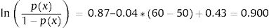
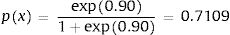


Consequently, in the first simulation (with Beta1*,Beta2*), the mean utility value for the subgroup of men aged 60, of high social status and a BMI <25 were calculated as:


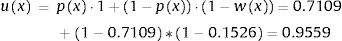
So, based on this regression model, 71.09% of the selected subpopulation was assumed in perfect health, and the estimated mean utility value for those not in perfect health was 0.8474 (= 1 − 0.1526). Therefore, the mean utility value for these specific characteristics was 0.9559 in the first simulation.
The procedure was then repeated with creation of new random vectors at the beginning of each simulation.
ConclusionsThe proposed approach allows, in the context of a model built for EE, the estimation of mean utility values based on individual characteristics. At the same time, it permits the inclusion of the associated uncertainty and ensures that the estimated value will always decrease in the interval −∞,1. In this way, second-order uncertainty related to mean utility values could be appropriately incorporated in cost-effectiveness simulation modelling.1
The proportion of individuals in perfect health can be a key factor when choosing the best methods for modelling utilities. According to the approach proposed by Briggs et al.,1 applying directly generalized linear models to 1−ux with log link will only be appropriate when individuals utility is lower than 1. Other authors, such as Basu and Manca,6 also suggested a two-step regression approach; however, a Beta distribution was assumed for the second step assuming negative mean utility values were not plausible. OLS models were suggested as the most unbiased approach by Pullenayegum et al.3 compared to the two-step model with normal or log-normal distribution in the second step. However, regarding to utilities conceptual definition, fitting the two-step procedure seems more adequate, even if might not always be the best approach to obtain the optimal point estimates.
When second order uncertainty is included in a model, using two-part models, coefficients estimated in the logistic model will be independent of the coefficients obtained in the second step. However, conceptually, all those parameters in the two-regression models should also be correlated. In fact, an existing zero-inflated regression approach10 would be useful for Poisson or negative binomial distributions, but further studies would be needed for other distributions such as log-normal distribution or gamma.
In this study we highlight the use of two-part models combined with variance-covariance matrix Cholesky decomposition as a generalized procedure that includes second-order uncertainty in covariate adjusted utilities to ensure the proper range, i.e. −∞,1, for all generated utility values.
Editor in chargeJuanjo Alguacil.
Authorship contributionsA. Arrospide, J.M. Ramos-Goñi and J. Mar conceived and designed the study. A. Arrospide, J.M. Ramos-Goñi and P. Pechlivanoglou performed the analysis of the data. A. Arrospide and J. Mar drafted the manuscript. All authors participated in the interpretation of the results, critically revised the manuscript for important intellectual content and have read and approved the final version of the manuscript.
AcknowledgmentsWe would like to acknowledge the English editorial assistance provided by Sally Ebeling.
FundingThis work was supported by grants from the Department of Health of Government of the Basque Country (File 201411107) and by grants from the Institute of Health Carlos III jointly funded by the European Fund for Regional Development – FEDER. Department of Health of Government of the Basque Country funded a collaborative stay at Sick Kids Hospital in Toronto (Canada) (File 2017011028).
Conflict of interestNone.