Researchers in public health are often interested in examining the effect of several exposures on the incidence of a recurrent event. The aim of the present study is to assess how well the common-baseline hazard models perform to estimate the effect of multiple exposures on the hazard of presenting an episode of a recurrent event, in presence of event dependence and when the history of prior-episodes is unknown or is not taken into account.
MethodsThrough a comprehensive simulation study, using specific-baseline hazard models as the reference, we evaluate the performance of common-baseline hazard models by means of several criteria: bias, mean squared error, coverage, confidence intervals mean length and compliance with the assumption of proportional hazards.
ResultsResults indicate that the bias worsen as event dependence increases, leading to a considerable overestimation of the exposure effect; coverage levels and compliance with the proportional hazards assumption are low or extremely low, worsening with increasing event dependence, effects to be estimated, and sample sizes.
ConclusionsCommon-baseline hazard models cannot be recommended when we analyse recurrent events in the presence of event dependence. It is important to have access to the history of prior-episodes per subject, it can permit to obtain better estimations of the effects of the exposures
A menudo los investigadores en salud pública están interesados en examinar el efecto de varias exposiciones en la incidencia de un evento recurrente. El objetivo de este estudio es evaluar el funcionamiento de los modelos de riesgo basal común al estimar el efecto de múltiples exposiciones sobre el riesgo de presentar un episodio de un evento recurrente, cuando existe dependencia del evento y los antecedentes de los episodios por sujeto son desconocidos o bien no se tienen en cuenta.
MétodosMediante un estudio exhaustivo de simulación, utilizando modelos de riesgo basal específico como referencia, se evalúa el rendimiento de los modelos de riesgo basal común a través de diversos criterios: sesgo, error cuadrático medio, cobertura, longitud de los intervalos de confianza y compatibilidad con el supuesto de riesgos proporcionales.
ResultadosEl sesgo empeora a medida que aumenta la dependencia del evento, llevando a una sobreestimación considerable del efecto de la exposición; los niveles de cobertura y el cumplimiento del supuesto de riesgos proporcionales son bajos o muy bajos, lo que empeora con el aumento de la dependencia del evento, el efecto a estimar y el tamaño muestral.
ConclusionesEl uso de modelos de riesgo basal común no puede recomendarse cuando analizamos eventos recurrentes en presencia de dependencia del evento. Es importante tener acceso a los antecedentes de episodios previos por sujeto, ya que ello puede permitir obtener mejores estimaciones de los efectos de las exposiciones.
The outcome of interest in a biomedical or epidemiological study is often an event that can occur more than once in a subject. Therefore, identifying a statistical method suitable for studying recurrent events is of great interest to the field.
From a statistical point of view, recurrent event analysis presents two major challenges. The first is individual heterogeneity, i.e. the unmeasured effects produced by between-subject variability, presumably due to unobserved exposures. For instance, imagine that a study measuring the number of respiratory crises is not asking for smoking status. It is likely that smokers will have a different pattern from non-smokers, resulting in heterogeneity across the subjects that can’t be attributed to any known factor as smoking status was not recorded. This issue is usually tackled using frailty models, which incorporate random effect terms to account for this “extra” variability. The second problem is within-subject correlations attributable to a single subject suffering multiple episodes of the event. These correlations are especially problematic in situations complicated by event dependence, in other words, when the risk of having a new episode depends on the number of previous episodes. This is the case of the number of sick leaves suffered by workers: A history of sick leaves increases the risk of a subsequent episode. Reis et al.1 quantified the extent of this increase. If we fail to account for event dependence, our resulting estimators will be inefficient and potentially biased. As discussed in Box-Steffensmeier et al.,2 common-baseline hazard models average the effects across all events not taking strata into account, being this averages biased in a predictable direction. In cohort studies, event dependence can be controlled by using survival models with specific-baseline hazards for each episode that the subject faces.3
Amorim and Cai4 provide an excellent review of approaches to recurrent event analysis. The article describes the applicable statistical methods for epidemiological studies of recurrent events, working off of the assumption that researchers have access to all of the information required by each model. In practice, however, much of this data is typically unavailable. Specific-baseline hazard models assume that the exact number of previous episodes suffered by each subject is known, but in reality it is typically impractical to obtain an exhaustive history for each patient. This leaves us without a method to directly address event dependence. The usual practice in such cases is to fit models with a common-baseline hazard.
The aim of the present study is to assess how well these common-baseline hazard models perform when they are used to estimate the effect of multiple exposures on the hazard of presenting an episode of a recurrent event when the previous history is not taken into account.
MethodsSimulationsExampleWe illustrate this work by reproducing a study from the literature5 to analyze long-term sickness absence (SA) frequency in a cohort of Dutch workers. We will use the same baseline hazard as in the Dutch study, 0.0021 per worker-week. The between-episodes hazard ratios (HR) do not correspond exactly to those of any specific study, although Reis et al.1 provide values for a wide range of SA-related diagnoses. SA is a commonly-used outcome in occupational health studies because it is considered a major economic and public health issue,6–8 resulting in a growing interest in identifying the best method to quantitatively and efficiently analyze this phenomenon.5,9–13
Generation of populationsSix different populations of 250 000 workers, each with 20 years of history, were generated using the survsim14,15 package in R 2.15.3 (R Foundation for Statistical Computing, Vienna, Austria). For each subject i, the hazard of the next episode k was simulated through an exponential distribution:
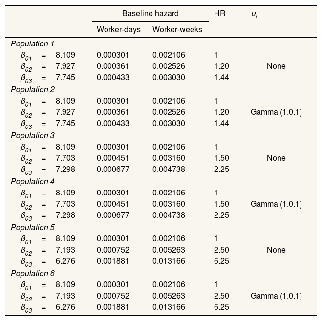
where h0kt=e−β0k, i.e. the baseline hazard for subjects exposed to episode k. The maximum number of SA episodes that a worker may suffer was not fixed, although the baseline hazard was considered constant when k≥3. X1, X2, and X3 are the three covariates that represent the exposure, with Xi∼Bernoulli (0.5). β1, β2, and β3 are the parameters of the three covariates that represent the effect, set independently of the episode k to which the worker is exposed, as: β1=0.25, β2=0.5, and β3=0.75 in order to represent effects of different magnitudes. νi is a random effect.Event dependenceEvent dependence was addressed by using various values of h0kt, specifying different β0k. Table 1 presents the specifications for the generated populations in terms of the baseline hazards by SA episode and random effects used. Table 1 also presents the HR resulting from the comparison of the baseline hazard with that of the first episode, which gives us the event dependence for the phenomenon. Note that for populations 1 and 2, the HR=1.20 and 1.44, respectively, for the second SA episode, as well as for the third and subsequent SA episodes with respect to the first. This means that between the second and third SA episodes, the baseline hazard was also increased by a factor of 1.20. The HR=1.50 between episodes two and three for populations 3 and 4, and 2.50 for populations 5 and 6. We chose to simulate phenomena with increasing event dependence, given that Reis et al.1 demonstrated that the hazard always increases in the presence of previous SA.
Characteristics of the simulated populations.
| Baseline hazard | HR | υi | ||
|---|---|---|---|---|
| Worker-days | Worker-weeks | |||
| Population 1 | ||||
| β01=8.109 | 0.000301 | 0.002106 | 1 | None |
| β02=7.927 | 0.000361 | 0.002526 | 1.20 | |
| β03=7.745 | 0.000433 | 0.003030 | 1.44 | |
| Population 2 | ||||
| β01=8.109 | 0.000301 | 0.002106 | 1 | Gamma (1,0.1) |
| β02=7.927 | 0.000361 | 0.002526 | 1.20 | |
| β03=7.745 | 0.000433 | 0.003030 | 1.44 | |
| Population 3 | ||||
| β01=8.109 | 0.000301 | 0.002106 | 1 | None |
| β02=7.703 | 0.000451 | 0.003160 | 1.50 | |
| β03=7.298 | 0.000677 | 0.004738 | 2.25 | |
| Population 4 | ||||
| β01=8.109 | 0.000301 | 0.002106 | 1 | Gamma (1,0.1) |
| β02=7.703 | 0.000451 | 0.003160 | 1.50 | |
| β03=7.298 | 0.000677 | 0.004738 | 2.25 | |
| Population 5 | ||||
| β01=8.109 | 0.000301 | 0.002106 | 1 | None |
| β02=7.193 | 0.000752 | 0.005263 | 2.50 | |
| β03=6.276 | 0.001881 | 0.013166 | 6.25 | |
| Population 6 | ||||
| β01=8.109 | 0.000301 | 0.002106 | 1 | Gamma (1,0.1) |
| β02=7.193 | 0.000752 | 0.005263 | 2.50 | |
| β03=6.276 | 0.001881 | 0.013166 | 6.25 | |
β03 refers to β0 for the third and subsequent episodes.
HR: hazard ratio.
Individual heterogeneity was addressed by introducing νi, the random effect. This effect was held constant over the various episodes for a given subject but varied between subjects. Specifically, we established: a) absence of any random effect νi=1, which leads to a perfectly specified population once the subject covariates are set, and b) individual heterogeneity, where νi∼Gamma with mean=1 and variance=0.1.
Table 1 shows the simulated populations.
Cohort designAlthough the populations with 20 years of history were generated, a procedure was subsequently applied to limit the effective follow-up periods to 1, 3, and 5 years, with some subjects having suffered a prior episode before the follow-up period began.
This was achieved as follows.
We selected the subjects who were either present at 15 years of follow-up or incorporated after that date. Follow-up time was then re-scaled, setting t=0 at 15 years for subjects already present in the population and t=0 at the beginning of the follow-up period for those incorporated later. The purpose of this procedure was to obtain a cohort in which some subjects had a work history prior to the 15-year point that included previous episodes, which were treated as unknown. The figure of 15 years was chosen as a representative length of work history for typical corporate employee. Using this subpopulation, we then generated the three sub-bases corresponding to different study end-points: at 16 years (1 year of effective follow-up, from the 15th to 16th year), at 18 years (three years of follow-up), and at 20 years (five years of follow-up).
Sample selection and model fittingFor each of sub-base, B=500 random samples were drawn with sizes n1=500, n2=1000, and n3=3000, and for each selected subject, the episodes within the effective follow-up period were recorded. Finally, the models were fitted to each of these samples.
ModelsAll of the models considered are non-parametric and are extensions of the Cox proportional hazards model.16,17 For all workers, we use the real previous episodes when fitting specific-baseline models, and we completely ignore them in the common-baseline models.
Models for non-individual heterogeneity context- 1)
Specific-baseline hazard approach: Prentice-Williams-Peterson (PWP)
For studies of recurrent phenomena involving event dependence but not individual heterogeneity, PWP is the survival model of reference.18 PWP addresses event dependence by stratifying according to number of previous episodes, thereby assigning a specific-baseline hazard to each potential episode. When the i-th subject is at risk of the k-th episode, the hazard function is defined as:
where Xiβ represent the vectors of covariates and the regression coefficients. - 2)
Common-baseline hazard approach: Andersen-Gill (AG)
AG19 is based on counting processes and assumes that the baseline hazard is common across all episodes, independent of the number of previous episodes. It has the following hazard function:
where h0t=e−β0 and is therefore the same for all episodes, k. AG treats different episodes within a given subject as though they were independent, subsequently obtaining a robust “sandwich” estimator of the variance.20
- 1)
Specific-baseline hazard approach: Conditional Frailty Model (CFM)
When individual heterogeneity comes into play, the reference model becomes CFM.21 This model addresses individual heterogeneity by assuming a latent multiplicative effect on the hazard function:
Ui is an individual random effect which is assumed to have unit mean and finite variance, which is estimated from the data.22 Since Ui is a multiplicative effect, we can think this frailty as a representation of the cumulative effect of one or more omitted covariates.22,23 The most commonly-adopted frailty terms24–26 are EUi=1 and VUi=θ.
- 2)
Common-baseline hazard approach: Shared Frailty Model (SFM)
Among other applications, SFM27–29 may be used in the context of recurrent events, where within-subject episodes share a frailty term that is independent of those for other individuals. Its hazard function is:
where the baseline hazard is independent of the episode k to which the subject is exposed. Ui is parameterized as in CFM.
The criteria used to evaluate model performance were: 1) percentage bias: δ=βˆ¯−ββ×100, where β is the true value for estimate of interest, βˆ¯=∑j=1BβˆjB, where B is the number of simulations performed; 2) percentage mean squared error (MSE): MSE=(βˆj−β)2+Vβˆjβ¯×100, for j=1,…,B, where βˆj is the estimate of interest within each of the j=1,…,B simulations and Vβˆj is the variance of the estimate of interest within each simulation; 3) coverage: percentage of times that the 95% confidence interval βˆj±z1−α/2SEβˆj includes β, for j=1,…,B, where SEβˆj is the standard error of the estimate of interest within each simulation; 4) confidence intervals average length; 5) proportional hazards: Percentage of times that the assumption of proportional hazards cannot be rejected, for j=1,…,B, according to the test proposed by Grambsch and Therneau.30
All models were fitted using the coxph function from the survival31 package in R.
ResultsThe results presented here refer only to the 5-year follow-up cohorts. Results for the cohorts with 1 and 3 years of follow-up are available as supplementary data online, but are not detailed here, as the findings were quite similar.
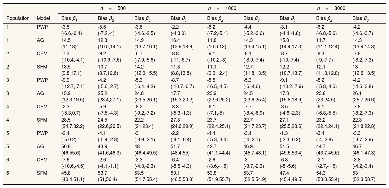
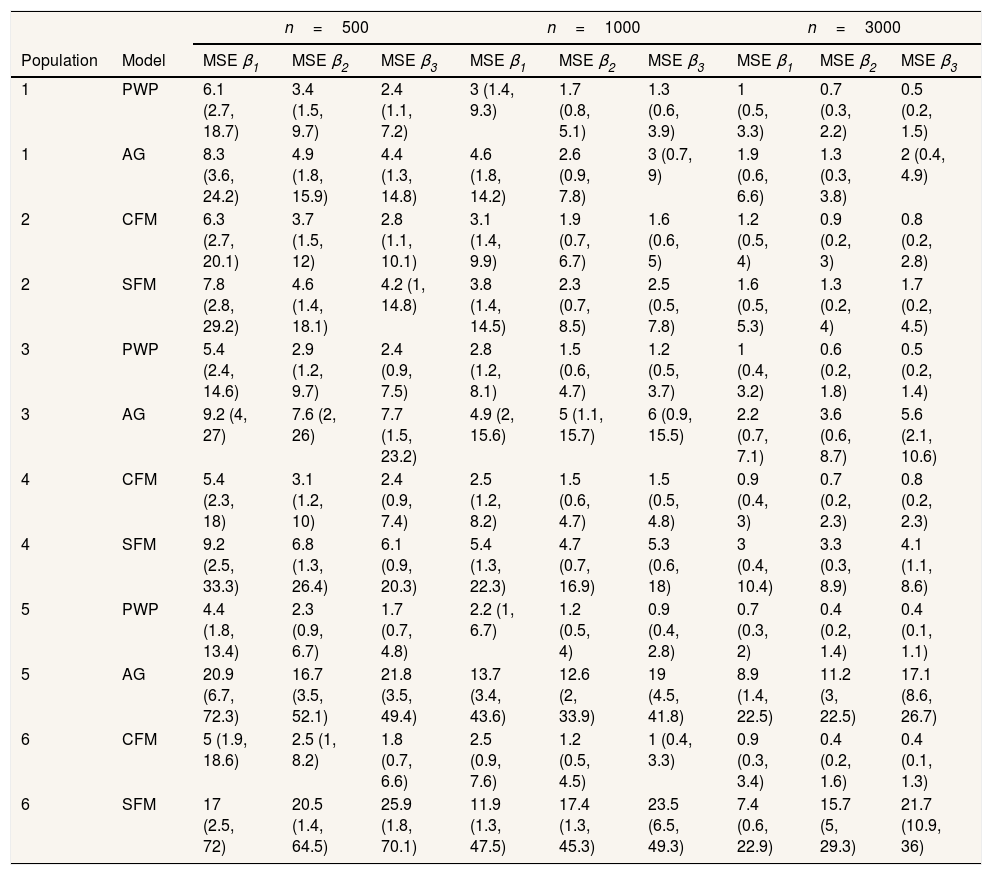
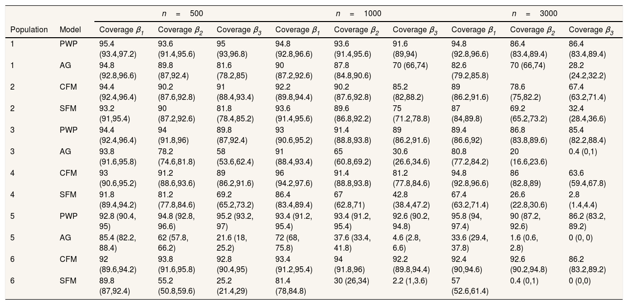
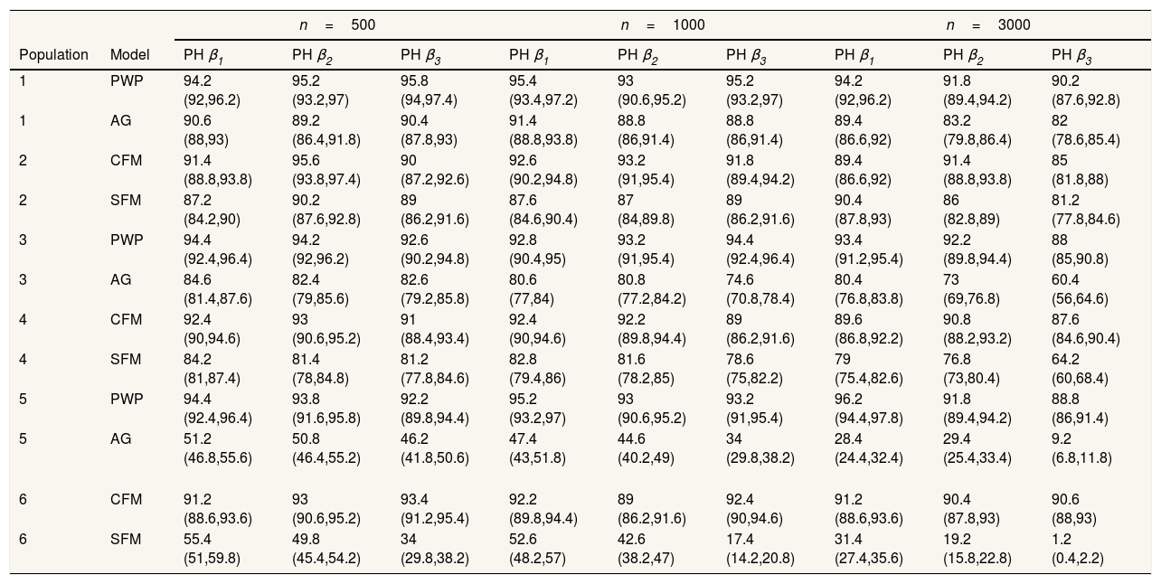
Regarding the situations with no-individual heterogeneity, we can see that the average bias in the common-baseline hazard models is 11−16% for population with low event dependence, rising to 42−51% for those with high event dependence (Table 2). In general, the bias does not change markedly in terms of the effect associated with β, sample size, or heterogeneity of the population. Higher sample size means lower MSE and, for common-baseline models, MSE increases with the exposure effect (Table 3). In terms of coverage, Table 4 shows that AG only achieves performances approaching 95% for populations with small or moderate event dependence (populations 1 and 3) and for β1=0.25. For the other scenarios, coverage falls notably, worsening with increasing event dependence, effect to estimate, and sample size. For example, in population 5, the 95%CI included the true parameter value for β3 in a mere 0-4.6% of samples when n=1000 or n=3000. As shown in Table 5, AG demonstrated overall low compliance with the assumption of proportional hazards, worsening with increasing event dependence, effect to estimate, and sample size. Compliance reached levels approaching 90% only in population 1, falling dramatically for population 5.
Percentage of bias (95% confidence interval).
| n=500 | n=1000 | n=3000 | ||||||||
|---|---|---|---|---|---|---|---|---|---|---|
| Population | Model | Bias β1 | Bias β2 | Bias β3 | Bias β1 | Bias β2 | Bias β3 | Bias β1 | Bias β2 | Bias β3 |
| 1 | PWP | -3.5 (-6.6,-0.4) | -5.6 (-7.2,-4) | -3.6 (-4.6,-2.5) | -2.2 (-4.3,0) | -6.2 (-7.2,-5.1) | -4.4 (-5.2,-3.6) | -3.1 (-4.4,-1.8) | -6.2 (-6.8,-5.6) | -4.2 (-4.6,-3.7) |
| 1 | AG | 14.5 (11,18) | 12.3 (10.5,14.1) | 14.9 (13.7,16.1) | 16.4 (13.9,18.9) | 11.8 (10.6,13) | 14.3 (13.4,15.1) | 15.8 (14.4,17.3) | 11.7 (11.1,12.4) | 14.3 (13.9,14.8) |
| 2 | CFM | -7.3 (-10.4,-4.1) | -9.2 (-10.9,-7.6) | -6.7 (-7.9,-5.6) | -8.8 (-11,-6.7) | -9.1 (-10.2,-8) | -8.1 (-8.9,-7.4) | -8.7 (-10,-7.4) | -8.3 (-9,-7.7) | -7.8 (-8.2,-7.3) |
| 2 | SFM | 13.5 (9.8,17.1) | 10.7 (8.7,12.6) | 14.2 (12.9,15.5) | 11.3 (8.8,13.8) | 11.1 (9.9,12.4) | 12.7 (11.8,13.5) | 12.2 (10.7,13.7) | 12.1 (11.3,12.8) | 13 (12.6,13.5) |
| 3 | PWP | -9.9 (-12.7,-7.1) | -4.2 (-5.6,-2.7) | -5.3 (-6.4,-4.2) | -8.7 (-10.7,-6.7) | -5.5 (-6.5,-4.5) | -5.3 (-6,-4.6) | -9.1 (-10.2,-7.9) | -5.2 (-5.8,-4.6) | -4.2 (-4.6,-3.8) |
| 3 | AG | 15.9 (12.3,19.5) | 25.2 (23.4,27.1) | 24.8 (23.5,26.1) | 17.7 (15.3,20.2) | 23.9 (22.6,25.2) | 24.5 (23.6,25.4) | 17.3 (15.8,18.9) | 23.8 (23,24.5) | 26.1 (25.7,26.6) |
| 4 | CFM | -2.3 (-5.3,0.7) | -5.9 (-7.5,-4.3) | -8.2 (-9.2,-7.2) | -3.3 (-5.3,-1.3) | -6.1 (-7.1,-5) | -7.7 (-8.4,-6.9) | -3.5 (-4.6,-2.3) | -6.1 (-6.8,-5.5) | -7.8 (-8.2,-7.3) |
| 4 | SFM | 28.5 (24.7,32.2) | 24.5 (22.6,26.5) | 22.2 (21,23.4) | 27.3 (24.6,29.9) | 23.7 (22.4,25.1) | 22.7 (21.7,23.7) | 27.1 (25.5,28.6) | 23.2 (22.4,24.1) | 22.3 (21.8,22.8) |
| 5 | PWP | -2.4 (-5,0.2) | -4.1 (-5.4,-2.8) | -3 (-3.9,-2.1) | -2.2 (-4.1,-0.4) | -4.4 (-5.3,-3.4) | -3.4 (-4,-2.7) | -1.3 (-2.3,-0.2) | -3.4 (-4,-2.8) | -3.3 (-3.7,-2.9) |
| 5 | AG | 50.8 (46,55.6) | 43.9 (41.6,46.3) | 48 (46.4,49.5) | 51.7 (48.4,55) | 42.7 (41.1,44.4) | 46.9 (45.7,48.1) | 51.5 (49.6,53.4) | 44.7 (43.7,45.6) | 46.7 (46.1,47.3) |
| 6 | CFM | -7.6 (-10.6,-4.6) | -2.6 (-4.1,-1.1) | -3.3 (-4.3,-2.3) | -6.4 (-8.5,-4.3) | -2.6 (-3.6,-1.6) | -3 (-3.7,-2.3) | -6.8 (-8,-5.6) | -2.1 (-2.7,-1.5) | -3.8 (-4.2,-3.4) |
| 6 | SFM | 45.8 (40.4,51.1) | 53.7 (51,56.4) | 53.5 (51.7,55.4) | 50.1 (46.5,53.8) | 53.8 (51.9,55.7) | 53.7 (52.5,54.9) | 47.4 (45.4,49.5) | 54.3 (53.3,55.4) | 53 (52.3,53.7) |
Percentage mean squared error (95% confidence interval).
| n=500 | n=1000 | n=3000 | ||||||||
|---|---|---|---|---|---|---|---|---|---|---|
| Population | Model | MSE β1 | MSE β2 | MSE β3 | MSE β1 | MSE β2 | MSE β3 | MSE β1 | MSE β2 | MSE β3 |
| 1 | PWP | 6.1 (2.7, 18.7) | 3.4 (1.5, 9.7) | 2.4 (1.1, 7.2) | 3 (1.4, 9.3) | 1.7 (0.8, 5.1) | 1.3 (0.6, 3.9) | 1 (0.5, 3.3) | 0.7 (0.3, 2.2) | 0.5 (0.2, 1.5) |
| 1 | AG | 8.3 (3.6, 24.2) | 4.9 (1.8, 15.9) | 4.4 (1.3, 14.8) | 4.6 (1.8, 14.2) | 2.6 (0.9, 7.8) | 3 (0.7, 9) | 1.9 (0.6, 6.6) | 1.3 (0.3, 3.8) | 2 (0.4, 4.9) |
| 2 | CFM | 6.3 (2.7, 20.1) | 3.7 (1.5, 12) | 2.8 (1.1, 10.1) | 3.1 (1.4, 9.9) | 1.9 (0.7, 6.7) | 1.6 (0.6, 5) | 1.2 (0.5, 4) | 0.9 (0.2, 3) | 0.8 (0.2, 2.8) |
| 2 | SFM | 7.8 (2.8, 29.2) | 4.6 (1.4, 18.1) | 4.2 (1, 14.8) | 3.8 (1.4, 14.5) | 2.3 (0.7, 8.5) | 2.5 (0.5, 7.8) | 1.6 (0.5, 5.3) | 1.3 (0.2, 4) | 1.7 (0.2, 4.5) |
| 3 | PWP | 5.4 (2.4, 14.6) | 2.9 (1.2, 9.7) | 2.4 (0.9, 7.5) | 2.8 (1.2, 8.1) | 1.5 (0.6, 4.7) | 1.2 (0.5, 3.7) | 1 (0.4, 3.2) | 0.6 (0.2, 1.8) | 0.5 (0.2, 1.4) |
| 3 | AG | 9.2 (4, 27) | 7.6 (2, 26) | 7.7 (1.5, 23.2) | 4.9 (2, 15.6) | 5 (1.1, 15.7) | 6 (0.9, 15.5) | 2.2 (0.7, 7.1) | 3.6 (0.6, 8.7) | 5.6 (2.1, 10.6) |
| 4 | CFM | 5.4 (2.3, 18) | 3.1 (1.2, 10) | 2.4 (0.9, 7.4) | 2.5 (1.2, 8.2) | 1.5 (0.6, 4.7) | 1.5 (0.5, 4.8) | 0.9 (0.4, 3) | 0.7 (0.2, 2.3) | 0.8 (0.2, 2.3) |
| 4 | SFM | 9.2 (2.5, 33.3) | 6.8 (1.3, 26.4) | 6.1 (0.9, 20.3) | 5.4 (1.3, 22.3) | 4.7 (0.7, 16.9) | 5.3 (0.6, 18) | 3 (0.4, 10.4) | 3.3 (0.3, 8.9) | 4.1 (1.1, 8.6) |
| 5 | PWP | 4.4 (1.8, 13.4) | 2.3 (0.9, 6.7) | 1.7 (0.7, 4.8) | 2.2 (1, 6.7) | 1.2 (0.5, 4) | 0.9 (0.4, 2.8) | 0.7 (0.3, 2) | 0.4 (0.2, 1.4) | 0.4 (0.1, 1.1) |
| 5 | AG | 20.9 (6.7, 72.3) | 16.7 (3.5, 52.1) | 21.8 (3.5, 49.4) | 13.7 (3.4, 43.6) | 12.6 (2, 33.9) | 19 (4.5, 41.8) | 8.9 (1.4, 22.5) | 11.2 (3, 22.5) | 17.1 (8.6, 26.7) |
| 6 | CFM | 5 (1.9, 18.6) | 2.5 (1, 8.2) | 1.8 (0.7, 6.6) | 2.5 (0.9, 7.6) | 1.2 (0.5, 4.5) | 1 (0.4, 3.3) | 0.9 (0.3, 3.4) | 0.4 (0.2, 1.6) | 0.4 (0.1, 1.3) |
| 6 | SFM | 17 (2.5, 72) | 20.5 (1.4, 64.5) | 25.9 (1.8, 70.1) | 11.9 (1.3, 47.5) | 17.4 (1.3, 45.3) | 23.5 (6.5, 49.3) | 7.4 (0.6, 22.9) | 15.7 (5, 29.3) | 21.7 (10.9, 36) |
Coverage: percentage of times that the true parameter value is included in the 95% confidence interval.
| n=500 | n=1000 | n=3000 | ||||||||
|---|---|---|---|---|---|---|---|---|---|---|
| Population | Model | Coverage β1 | Coverage β2 | Coverage β3 | Coverage β1 | Coverage β2 | Coverage β3 | Coverage β1 | Coverage β2 | Coverage β3 |
| 1 | PWP | 95.4 (93.4,97.2) | 93.6 (91.4,95.6) | 95 (93,96.8) | 94.8 (92.8,96.6) | 93.6 (91.4,95.6) | 91.6 (89,94) | 94.8 (92.8,96.6) | 86.4 (83.4,89.4) | 86.4 (83.4,89.4) |
| 1 | AG | 94.8 (92.8,96.6) | 89.8 (87,92.4) | 81.6 (78.2,85) | 90 (87.2,92.6) | 87.8 (84.8,90.6) | 70 (66,74) | 82.6 (79.2,85.8) | 70 (66,74) | 28.2 (24.2,32.2) |
| 2 | CFM | 94.4 (92.4,96.4) | 90.2 (87.6,92.8) | 91 (88.4,93.4) | 92.2 (89.8,94.4) | 90.2 (87.6,92.8) | 85.2 (82,88.2) | 89 (86.2,91.6) | 78.6 (75,82.2) | 67.4 (63.2,71.4) |
| 2 | SFM | 93.2 (91,95.4) | 90 (87.2,92.6) | 81.8 (78.4,85.2) | 93.6 (91.4,95.6) | 89.6 (86.8,92.2) | 75 (71.2,78.8) | 87 (84,89.8) | 69.2 (65.2,73.2) | 32.4 (28.4,36.6) |
| 3 | PWP | 94.4 (92.4,96.4) | 94 (91.8,96) | 89.8 (87,92.4) | 93 (90.6,95.2) | 91.4 (88.8,93.8) | 89 (86.2,91.6) | 89.4 (86.6,92) | 86.8 (83.8,89.6) | 85.4 (82.2,88.4) |
| 3 | AG | 93.8 (91.6,95.8) | 78.2 (74.6,81.8) | 58 (53.6,62.4) | 91 (88.4,93.4) | 65 (60.8,69.2) | 30.6 (26.6,34.6) | 80.8 (77.2,84.2) | 20 (16.6,23.6) | 0.4 (0,1) |
| 4 | CFM | 93 (90.6,95.2) | 91.2 (88.6,93.6) | 89 (86.2,91.6) | 96 (94.2,97.6) | 91.4 (88.8,93.8) | 81.2 (77.8,84.6) | 94.8 (92.8,96.6) | 86 (82.8,89) | 63.6 (59.4,67.8) |
| 4 | SFM | 91.8 (89.4,94.2) | 81.2 (77.8,84.6) | 69.2 (65.2,73.2) | 86.4 (83.4,89.4) | 67 (62.8,71) | 42.8 (38.4,47.2) | 67.4 (63.2,71.4) | 26.6 (22.8,30.6) | 2.8 (1.4,4.4) |
| 5 | PWP | 92.8 (90.4, 95) | 94.8 (92.8, 96.6) | 95.2 (93.2, 97) | 93.4 (91.2, 95.4) | 93.4 (91.2, 95.4) | 92.6 (90.2, 94.8) | 95.8 (94, 97.4) | 90 (87.2, 92.6) | 86.2 (83.2, 89.2) |
| 5 | AG | 85.4 (82.2, 88.4) | 62 (57.8, 66.2) | 21.6 (18, 25.2) | 72 (68, 75.8) | 37.6 (33.4, 41.8) | 4.6 (2.8, 6.6) | 33.6 (29.4, 37.8) | 1.6 (0.6, 2.8) | 0 (0, 0) |
| 6 | CFM | 92 (89.6,94.2) | 93.8 (91.6,95.8) | 92.8 (90.4,95) | 93.4 (91.2,95.4) | 94 (91.8,96) | 92.2 (89.8,94.4) | 92.4 (90,94.6) | 92.6 (90.2,94.8) | 86.2 (83.2,89.2) |
| 6 | SFM | 89.8 (87,92.4) | 55.2 (50.8,59.6) | 25.2 (21.4,29) | 81.4 (78,84.8) | 30 (26,34) | 2.2 (1,3.6) | 57 (52.6,61.4) | 0.4 (0,1) | 0 (0,0) |
Percentage of times that the assumption of proportional hazards is not rejected (95% confidence interval).
| n=500 | n=1000 | n=3000 | ||||||||
|---|---|---|---|---|---|---|---|---|---|---|
| Population | Model | PH β1 | PH β2 | PH β3 | PH β1 | PH β2 | PH β3 | PH β1 | PH β2 | PH β3 |
| 1 | PWP | 94.2 (92,96.2) | 95.2 (93.2,97) | 95.8 (94,97.4) | 95.4 (93.4,97.2) | 93 (90.6,95.2) | 95.2 (93.2,97) | 94.2 (92,96.2) | 91.8 (89.4,94.2) | 90.2 (87.6,92.8) |
| 1 | AG | 90.6 (88,93) | 89.2 (86.4,91.8) | 90.4 (87.8,93) | 91.4 (88.8,93.8) | 88.8 (86,91.4) | 88.8 (86,91.4) | 89.4 (86.6,92) | 83.2 (79.8,86.4) | 82 (78.6,85.4) |
| 2 | CFM | 91.4 (88.8,93.8) | 95.6 (93.8,97.4) | 90 (87.2,92.6) | 92.6 (90.2,94.8) | 93.2 (91,95.4) | 91.8 (89.4,94.2) | 89.4 (86.6,92) | 91.4 (88.8,93.8) | 85 (81.8,88) |
| 2 | SFM | 87.2 (84.2,90) | 90.2 (87.6,92.8) | 89 (86.2,91.6) | 87.6 (84.6,90.4) | 87 (84,89.8) | 89 (86.2,91.6) | 90.4 (87.8,93) | 86 (82.8,89) | 81.2 (77.8,84.6) |
| 3 | PWP | 94.4 (92.4,96.4) | 94.2 (92,96.2) | 92.6 (90.2,94.8) | 92.8 (90.4,95) | 93.2 (91,95.4) | 94.4 (92.4,96.4) | 93.4 (91.2,95.4) | 92.2 (89.8,94.4) | 88 (85,90.8) |
| 3 | AG | 84.6 (81.4,87.6) | 82.4 (79,85.6) | 82.6 (79.2,85.8) | 80.6 (77,84) | 80.8 (77.2,84.2) | 74.6 (70.8,78.4) | 80.4 (76.8,83.8) | 73 (69,76.8) | 60.4 (56,64.6) |
| 4 | CFM | 92.4 (90,94.6) | 93 (90.6,95.2) | 91 (88.4,93.4) | 92.4 (90,94.6) | 92.2 (89.8,94.4) | 89 (86.2,91.6) | 89.6 (86.8,92.2) | 90.8 (88.2,93.2) | 87.6 (84.6,90.4) |
| 4 | SFM | 84.2 (81,87.4) | 81.4 (78,84.8) | 81.2 (77.8,84.6) | 82.8 (79.4,86) | 81.6 (78.2,85) | 78.6 (75,82.2) | 79 (75.4,82.6) | 76.8 (73,80.4) | 64.2 (60,68.4) |
| 5 | PWP | 94.4 (92.4,96.4) | 93.8 (91.6,95.8) | 92.2 (89.8,94.4) | 95.2 (93.2,97) | 93 (90.6,95.2) | 93.2 (91,95.4) | 96.2 (94.4,97.8) | 91.8 (89.4,94.2) | 88.8 (86,91.4) |
| 5 | AG | 51.2 (46.8,55.6) | 50.8 (46.4,55.2) | 46.2 (41.8,50.6) | 47.4 (43,51.8) | 44.6 (40.2,49) | 34 (29.8,38.2) | 28.4 (24.4,32.4) | 29.4 (25.4,33.4) | 9.2 (6.8,11.8) |
| 6 | CFM | 91.2 (88.6,93.6) | 93 (90.6,95.2) | 93.4 (91.2,95.4) | 92.2 (89.8,94.4) | 89 (86.2,91.6) | 92.4 (90,94.6) | 91.2 (88.6,93.6) | 90.4 (87.8,93) | 90.6 (88,93) |
| 6 | SFM | 55.4 (51,59.8) | 49.8 (45.4,54.2) | 34 (29.8,38.2) | 52.6 (48.2,57) | 42.6 (38.2,47) | 17.4 (14.2,20.8) | 31.4 (27.4,35.6) | 19.2 (15.8,22.8) | 1.2 (0.4,2.2) |
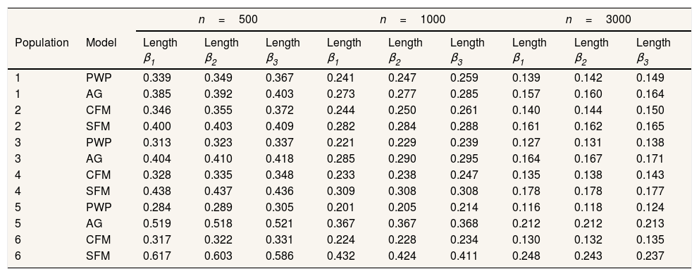
Results for heterogeneous populations present an almost identical pattern. Slight differences are observed regarding the 95%CI: SFM CI95% was generally broader (Table 6), translating into a slight rise in coverage level (Table 4).
Confidence intervals mean length.
| n=500 | n=1000 | n=3000 | ||||||||
|---|---|---|---|---|---|---|---|---|---|---|
| Population | Model | Length β1 | Length β2 | Length β3 | Length β1 | Length β2 | Length β3 | Length β1 | Length β2 | Length β3 |
| 1 | PWP | 0.339 | 0.349 | 0.367 | 0.241 | 0.247 | 0.259 | 0.139 | 0.142 | 0.149 |
| 1 | AG | 0.385 | 0.392 | 0.403 | 0.273 | 0.277 | 0.285 | 0.157 | 0.160 | 0.164 |
| 2 | CFM | 0.346 | 0.355 | 0.372 | 0.244 | 0.250 | 0.261 | 0.140 | 0.144 | 0.150 |
| 2 | SFM | 0.400 | 0.403 | 0.409 | 0.282 | 0.284 | 0.288 | 0.161 | 0.162 | 0.165 |
| 3 | PWP | 0.313 | 0.323 | 0.337 | 0.221 | 0.229 | 0.239 | 0.127 | 0.131 | 0.138 |
| 3 | AG | 0.404 | 0.410 | 0.418 | 0.285 | 0.290 | 0.295 | 0.164 | 0.167 | 0.171 |
| 4 | CFM | 0.328 | 0.335 | 0.348 | 0.233 | 0.238 | 0.247 | 0.135 | 0.138 | 0.143 |
| 4 | SFM | 0.438 | 0.437 | 0.436 | 0.309 | 0.308 | 0.308 | 0.178 | 0.178 | 0.177 |
| 5 | PWP | 0.284 | 0.289 | 0.305 | 0.201 | 0.205 | 0.214 | 0.116 | 0.118 | 0.124 |
| 5 | AG | 0.519 | 0.518 | 0.521 | 0.367 | 0.367 | 0.368 | 0.212 | 0.212 | 0.213 |
| 6 | CFM | 0.317 | 0.322 | 0.331 | 0.224 | 0.228 | 0.234 | 0.130 | 0.132 | 0.135 |
| 6 | SFM | 0.617 | 0.603 | 0.586 | 0.432 | 0.424 | 0.411 | 0.248 | 0.243 | 0.237 |
The specific-baseline hazard approaches showed much better results than the common-baseline approaches, both in homogeneous and heterogeneous contexts. For populations free of heterogeneity, the percentage of bias remained below 10% and was generally negative, i.e. slightly underestimating the effect and coverage levels were around 85−95%. Overall, more than 90% of the simulated samples complied with the assumption of proportional hazards. In presence of individual heterogeneity, when there is low event dependence, the bias slightly falls with the increase of the effect to estimate and sample size.
DiscussionStatistical analysis of recurrent outcomes with event dependence is not trivial, as it requires methods that can account for this dependence to obtain efficient and unbiased estimates. Although including the number of previous episodes as a time-dependent covariate would address the problem,10 episode-specific hazard functions are more coherent with the nature of recurrent events. In any case, to deploy either alternative, it is necessary to know how many previous episodes each subject has had, which is often impossible. As a result, some epidemiologists often recur to a common-baseline hazard function that is independent of previous episodes. The present paper assesses how well these common-baseline hazard models perform, in comparison to some of the most common specific-baseline hazard models, when applied to situations complicated by event dependence and when the previous episodes are not taken into account.
It is worth noting that the results obtained here may be indicative of the behavior of phenomena with “positive” event dependence (risk of presenting a new episode increases in function of the number of previous episodes), not when event dependence is “negative” (which in our opinion is much less common in the study of public health phenomena). Similarly, the magnitude of the bias, coverage levels, etc., depends on other specific aspects of each study, as the intensity of the event dependence, sample size, etc.
It is important to highlight that there were almost no differences between the pattern of behavior of common-baseline approach versus specific-baseline approach, in heterogeneous or homogenous populations in terms of bias, coverage, or compliance with the proportional hazards assumption.
The performance of the common-baseline approaches worsened as event dependence increased, producing lower coverage and increasingly overestimating the effect. Subjects in the previously-exposed group had more event occurrences and therefore more recurrent episodes, and they suffered these episodes earlier than subjects in the non-exposed group. Thus, the exposed subjects arrived at a higher baseline hazard sooner and in greater numbers. This means that if specific-baseline hazards are not used, the increased baseline hazard would be largely attributable to the exposed group.
As the effect to be estimated increases, performance of models with common-baseline hazard worsens. The explanation is similar to the one above: the larger the effect, the greater the difference in risk between subjects in exposed and non-exposed groups; hence, the numbers and recurrence rates among exposed subjects become progressively greater compared to those of the unexposed subjects. Thus, as in the case of event dependence, the baseline hazard effect is disproportionally attributable to exposure.
For these models, coverage is affected by sample size, worsening as sample size increases. Clearly this is a spurious relationship; what really happens is that larger sample sizes provide greater precision, but since the estimates obtained are biased, greater precision means poorer coverage.32
As expected, PWP was clearly superior to AG in situations complicated by event dependence. Even so, coverage and compliance with the proportional hazards assumption remained unacceptably low in the face of significant event dependence and large effects to be estimated. Note, however, that our results show that PWP overall tends to slightly underestimate the value of β. This is probably because the upper strata, representing subjects with greater numbers of recurrences, concentrate members of the exposed group. Further studies to investigate the best strategy to use in the upper strata would be helpful. In order to keep all episodes in the analysis, we pooled all episodes beyond the second recurrence. It would be interesting to see whether “truncating” the number of episodes or, alternatively, not grouping them together at all, would improve performance. The first option has the disadvantage of eliminating some episodes, whereas the second produces strata with very few subjects and consequently unstable estimates.27 All the above comments are also valid for CFM. On the other hand, Torá-Rocamora et al.13 show that fitting the CFM when dealing with very large datasets may require high computing times. In this case, a suitable alternative could be the conditional frailty Poisson model which produces similar results but decreases the time substantially. We should also mention that the approaches presented in this paper are not the only ones that could be used for the analysis of recurrent events. Alternatives include multilevel mixed effects survival parametric models33, flexible parametric34 or multistate models.35
In summary, information about previous episodes is fundamental for sound analysis of recurrent events, but the required data is not always available. All the common-baseline hazard models that we evaluated performed almost equally poorly, making it impossible to recommend one over another. The one exception in which a common-baseline hazard model may be a reasonable option for event-dependent analysis is a situation in which the level of event dependence is very low and the effect to be estimated is small. Although this estimate would still be somewhat biased, coverage and compliance with the proportional hazards assumption might be within the realm of acceptability. In other situations, these models are clearly inappropriate, producing low coverage, low or extremely low compliance with the proportional hazards assumption, and blatant overestimation of the effect of exposure. In practice, the magnitude of this problem may even be greater. Reis et al.1 showed that event dependence for SA is often higher than the figures used in our simulations, meaning that the common-baseline hazards models would perform even more poorly. The authors showed, for example, that the HR for the second and third episodes of sick leave due to mental and behavioral disorders were 9.52 and 20.26, respectively, with respect to the first episode.
From this paper we may derive two main conclusions: first, availability of the history of previous episodes per subject is very important and therefore, an effort to this purpose should be made in the fieldwork; second, if we don’t have this information, it is important to find valid alternatives to tackle analyses of this type. One option that we consider worth investigating is imputing the number of previous episodes, which would allow for the use of models with specific-hazard functions.
One of the main challenges in recurrent event analysis is accounting for within-subject correlations. Failure to properly address these correlations can create serious problems, especially in the presence of event dependence; that is, when the risk of having a new episode depends on the number of previous episodes suffered by the subject. The specific-baseline hazard model can be used to address event dependence and obtain efficient estimators. However, using a specific-baseline hazard model requires knowing the number of previous episodes experienced by each subject; in practice, these data is often unavailable. Under this situation, many researchers choose to use common-baseline hazard models to analyse this kind of data.
What does this study add to the literature?This study provides a quantification of the magnitude of the consequences of using common-baseline hazard models when there is event dependence, in several scenarios based on a realistic example. In this context, a common-baseline hazard model is not appropriate, as the model produces inefficient and biased estimations. The true parameter value does not fall within the confidence interval at an acceptable frequency, and compliance with the assumption of proportional hazards is unacceptably low.
María-Victoria Zunzunegui.
Transparency declarationThe corresponding author on behalf of the other authors guarantee the accuracy, transparency and honesty of the data and information contained in the study, that no relevant information has been omitted and that all discrepancies between authors have been adequately resolved and described.
Authorship contributionsAll authors contributed to the conception and design of the work, the design of the simulations, the analysis and interpretation of the data, the writing of the paper and its critical review with important intellectual contributions, and to the approval of the final version for its publications.
FundingNone.
Conflicts of interestsNone.


