To analyse the impact of per capita income and environmental air quality variables on health expenditure determinants.
MethodIn this study, we analyse the relationship between air pollution and health expenditure in 29 OECD countries over the period 1995-2014. In addition, we test whether our findings differ between countries with higher or lower incomes.
ResultsThe econometric results show that per capita income has a positive effect on health expenditure, but is not as statistically significant as expected when lag-time is incorporated. In addition, an anchorage effect is observed, which implies that about 80%-90% of previous expenditure explain current expenditure. Our empirical results are quite consistent between groups and when compared with the full sample. Nevertheless, there appear to be some differences when broken down by financing scheme (total, public, and private).
ConclusionsOverall, our findings could be used to clarify the appropriate health expenditure level or to obtain better environmental quality and social well-being. That is, empirical support is provided on how health management and policy makers should include more considerations for the use of cleaner fuels in developed countries.
Estudiar el impacto que tienen la renta per cápita y las variables de calidad ambiental sobre los gastos sanitarios.
MétodoAnalizamos la relación entre la contaminación atmosférica y el gasto sanitario en 29 países de la OCDE durante el periodo 1995-2014. Además, estudiamos si nuestros hallazgos difieren según los países (con ingresos más altos o más bajos).
ResultadosLos resultados econométricos muestran que la renta per cápita tiene un efecto positivo en los gastos sanitarios, pero no tan estadísticamente significativo como se esperaba al incorporar demoras. Además, se aprecia un efecto de anclaje, el cual implica que alrededor del 80-90% de los gastos anteriores explican los actuales. Nuestros resultados empíricos son bastante concordantes entre los grupos considerados, al compararse estos con la muestra completa. Sin embargo, parecen existir algunas diferencias al desglosar por tipo de financiación (total, pública y privada).
ConclusiónEn general, nuestros hallazgos podrían utilizarse para esclarecer el nivel adecuado de gasto sanitario, o bien para obtener una mejor calidad ambiental y bienestar social. Es decir, se brinda apoyo empírico sobre cómo la Administración (sanitaria) y los responsables de las distintas políticas públicas deberían incluir más consideraciones para el uso de combustibles más limpios en los países desarrollados.
Nowadays, there is an extensive literature focused on the determinants of health expenditures, being income the main one.1 However, non-income factors like the health care model, population and ageing dynamics, population lifestyles, the technological progress or the environmental determinants have been also identified.2 Indeed, there are both demand and supply factors that explain health expenditures dynamics. In this study, we focus on environmental issues that are very much in vogue these days.3–5 Precisely, we look forward to answering the following question: does air pollution affect health care expenditures? Nowadays, many of the most important researchers are grappling with how best to characterize the effects of environmental air quality, in order to help regulators and decision makers craft more-effective policies, to address both health and environmental issues in a context of scarce resources.
What is it well known is that air pollution is responsible for many adverse effects on health and well-being.6 Hence, air pollution, both referring household air pollution and ambient air pollution, is considered one of the great silent environmental killers these days.7 Actually, air pollution is a major cause of non-communicable diseases that should be taken into account to a greater extent.8 Moreover, ambient air pollution, in which we focus in this paper, is responsible for countless economic losses.9 Mainly, associated with health care utilization and so, health expenditures. But also, lost or delayed production due to absence from work.
Then, as pointed by Eckelman and Sherman10 new efforts to improve environmental performance of health care could reduce expenditures directly and indirectly. That is, by waste reduction and energy savings, and through reducing pollution burden on public health, these factors ought to be included in efforts to improve health care quality and safety. Indeed, as pointed by Pascal et al.11 European citizens are still exposed to concentrations exceeding the World Health Organization recommendations. These authors by the Aphekom Project provide robust estimates confirming that reducing urban air pollution would result in significant health and monetary gains. Moreover, by studying the public health impacts of urban air pollution in 25 European cities, they estimated a monetary gain around €31 billion annually, including savings on health expenditures, absenteeism and intangible costs such as well-being, life expectancy and quality of life.
Based on these previous assumptions, the general aim of our study is to expand the analysis of the determinants of health expenditures. We analyse the relationship between health expenditures and income at the aggregate level, by providing some updates on previous related studies for developed countries and incorporating environmental factors. Besides, most of the studies make use as health expenditure variable the total health expenditure made by each country, we also distinguish between public and private ones.
Precisely, this study exploits a balanced dataset of 29 OECD selected countries during the period 1995-2014. Moreover, a cluster analysis based on the heterogeneity of our sample selected is also performed. Then, from a first specification in line with the main articles on the subject, we introduce the described novelties, where the dependent variable is always the logarithm of per capita total health care expenditures, but considering several health care financing schemes. In doing so, we first assume a linear and homogeneous relationship between income, environmental factors and health expenditures. Nevertheless, at the end, we also consider a dynamic model following the line proposed by Lago-Peñas et al.12
Therefore, the main contribution of this paper is the use of recently data and the introduction of new variables in the estimates that make a new image of the traditional studies in order to provide support about how health management and policy makers should include new insights for the use of cleaner fuels in developed countries. Indeed, this research line of international studies by analysing complex relationships among air pollutants and health (and how it varies across territories) could improve public health and reduce inequalities in developed countries. That is, our results highlight that it is more crucial than ever to carry out an appropriate policy analysis at the macroeconomic level, which will allow policymakers to better allocate scarce resources.
MethodsDataExisting studies have examined different aspects of health expenditure determinants. Here we focus on environmental ones.3 In order to work with a complete balanced panel data, in this study our temporal analysis period is 1995-2014 for a selected group of 29 OECD countries namely: Australia, Austria, Belgium, Canada, Czech Republic, Denmark, Finland, France, Germany, Greece, Hungary, Iceland, Ireland, Italy, Japan, Latvia, Luxembourg, Netherlands, New Zealand, Norway, Poland, Portugal, Slovenia, Spain, Sweden, Switzerland, Turkey, United Kingdom, and the United States. The benefits of using a balanced panel data set consist in that it allows doing the analysis of stationarity of the variables. Besides, most of the tests require that the panels be strongly balanced.13
The econometric analysis relies on annual data obtained from two different data sources: the latest versions of OECD Health Statistics and OECD Environment Statistics. Information about per capita health care expenditures (total, public and private ones) and per capita GDP are measured at Purchasing Power Parity (PPPs) terms. Sulphur oxide emissions, nitrogen oxide emissions, and carbon monoxide emissions are in kilos per capita. All variables are converted into natural logarithmic form before the empirical analysis. The definition of the variables and summary statistics finally considered are described in Table I in the online Appendix.
This research provides rigorous scientific examinations to study the following issue: how air quality indicators affect health expenditures. Taking into account previous analysis, a positive relationship between income and health expenditures is expected. Additionally, we hypothesized that su, ni, and ca would also increase health expenditures.
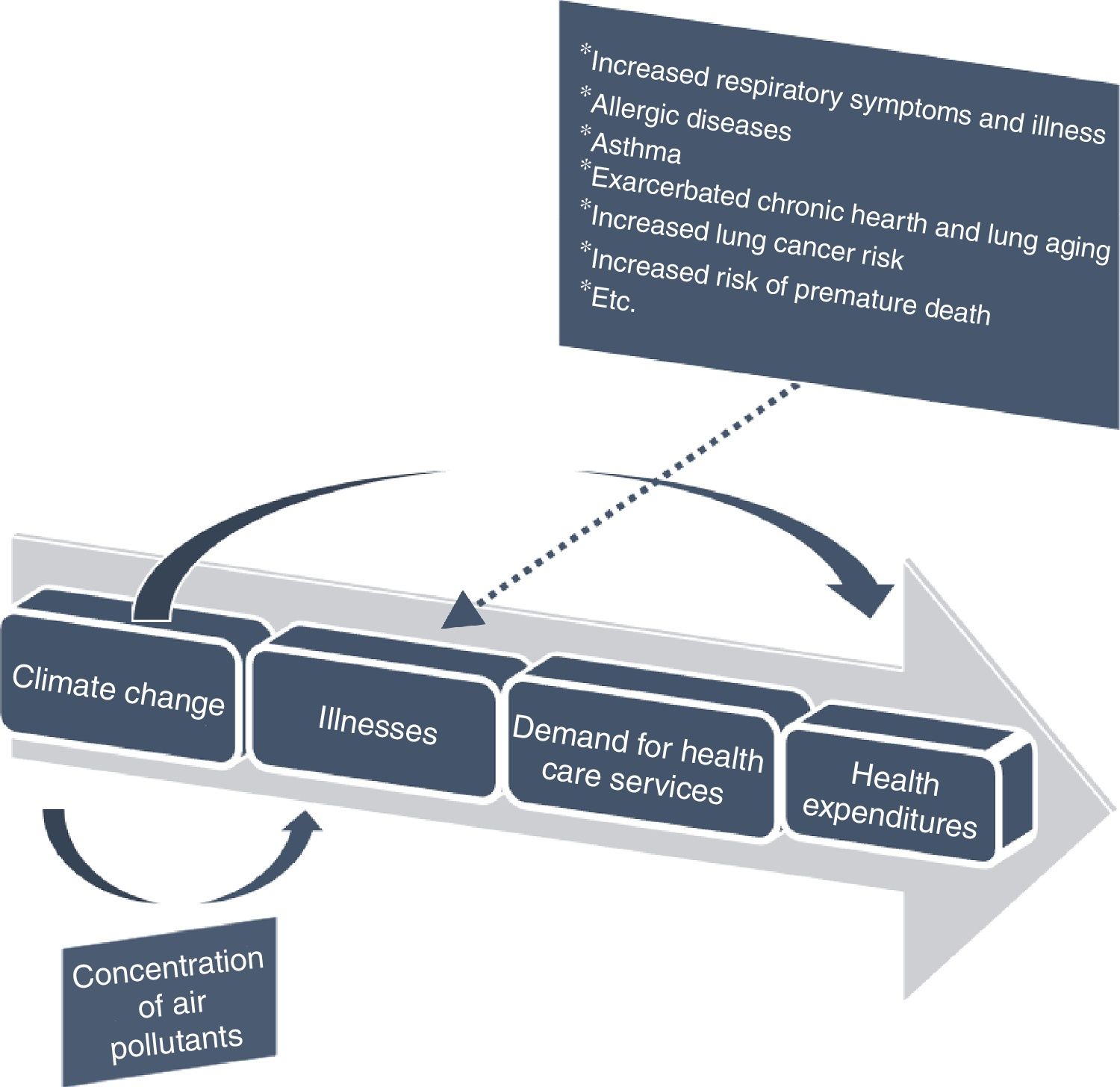
Figure 1 represents the pathway effects of climate change on health endpoint, because it may affect the exposures to air pollutants. In any case, pollution could appear by both natural and human sources. Here it is modelled how air, that could be contaminated with pollutants, may negatively affect health in general and health expenditures in particular. Thus, the health effects of air pollution are diverse, and include direct and indirect ones. All in all, the most sensitive groups include children, older adults and people with chronic heart or lung disease). The explanation is based on the idea that these three air pollutants measures here considered deteriorate air quality and so, they would affect negatively health outcomes.14
Pathway effects of climate change on health endpoint. (Authors’ elaboration adapted from Bernard et al.15).
Moreover, as pointed by Bernard et al.,15 health effects of exposures to sulphur and nitrogen oxides, and carbon monoxides, can cause reduced work capacity, aggravation of existing cardiovascular diseases, effects on pulmonary function, respiratory illnesses, lung irritation, and alterations in the lung's defence systems. That is, an increase in utilization (demand) of health care services due to bad health care outcomes is projected.
These interesting findings could be used to derive the appropriate health expenditure level, to obtain better environmental quality, and social well-being. Research needs considering air pollution models (and their potential linkage with climate change scenarios) in order to close gaps in the understanding of the relationship between air pollution exposure and health effects. In any case, health management and policy makers should consider these relationships.
Statistical approachOverall, we follow recent contributions, which consider the modelling advance of the relationship between health and environmental issues as Narayan and Narayan3 or Qureshi et al.16 Our empirical results are based on the following specifications with all the variables of interest are converted in natural logarithms form to allow us to understand them as elasticities.
Firstly, a linear one-way panel data model for health expenditure (he), as dependent variable to be analysed (while considering different measures of it depending on its source of financing: total, public, and private) based on the acknowledged literature is specified.17,18 Therefore, when income changes the variation in health care expenditure it is likely to be a combination of multiple forces. It is very useful to isolate these effects to gain enhanced insights into several components. In a more formal way, our model has the following general form:
where heit is the logarithm of per capita health care expenditures at the tth observation for the ith country; f(•) denotes health care expenditure structure; xit is the corresponding matrix of explanatory variables; β is a vector of parameters to be estimated (su, ni, ca and gdp). The term ɛ is the error bounded with the general statistical properties. Besides, feasible generalized least squares are considered. This procedure allows estimation in presence of first-order autocorrelation within panels and cross-sectional correlation, and heteroscedasticity across panels.
Secondly, a dynamic panel data approach is applied. That is, we include on the right-hand side of equation (1) the lagged dependent variable, in order to capture the inertia of health care expenditures. In other words, we try to disentangle if the logarithm of per capita health care expenditures on a year is conditioned by the previous one:
ResultsPreliminary testBefore presenting the results from the estimation of the above-mentioned specifications, we first analyse all variables to ensure accurate estimates. That is, to obtain empirical findings that are not spurious and have economic sense. Precisely, first and second generation of panel unit root tests are employed here. Tables II and III in the online Appendix show this type of tests. Firstly, we applied panel unit root tests assuming cross-sectional independence. Regarding Levin et al.19 and Im et al.20, mixed results concerning variables being stationary are showed. Statistic for the logarithm of our variables when the ADF regression has an intercept only and an intercept and a linear time trend, are presented. Nevertheless, a common feature of these econometric tests is that they lose power as individual specific trends are included.13 In all cases, the lag order p, was selected using the Akaike information criterion. Then, we also apply the Breitung21 test that indicates the hypothesis that variables contains unit root is never rejected. Considering all of this, we turned to Pesaran22 second generation test that attempts to remove cross-sectional dependence. We present results for lag orders p = 0, 1, 2 and 3, finding that in most of the cases our variables of interest are integrated of order 1, I(1).
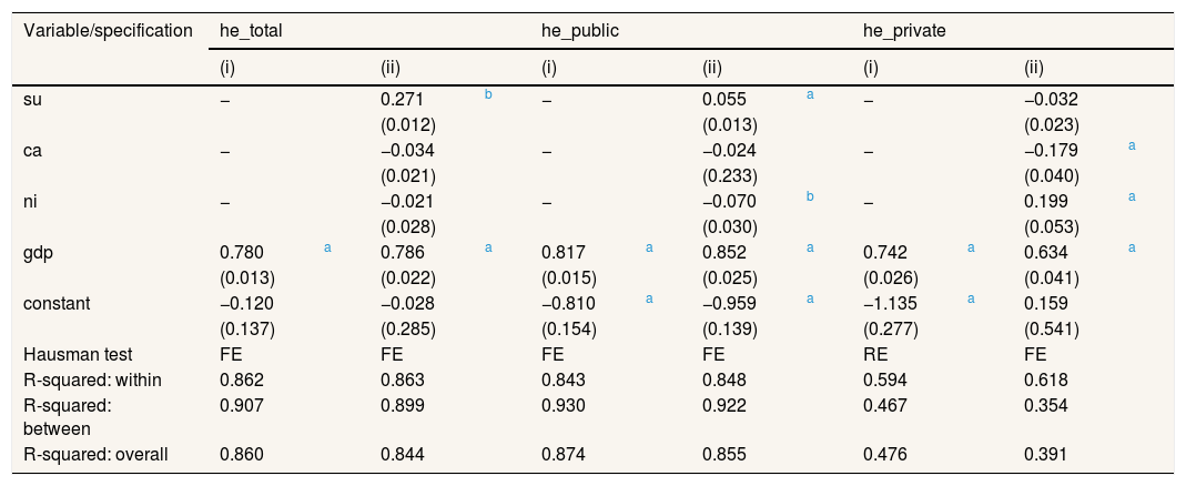
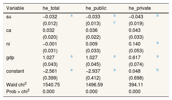
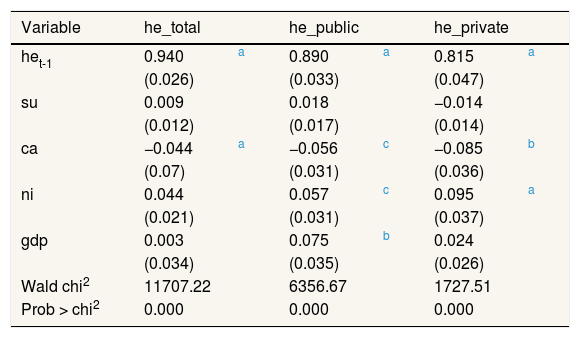
Empirical resultsThe estimation of the specification described yields the results reported in Tables 1-4. The first two tables considering (1) whereas the latest (2). Coefficients are highly significant, and the goodness of fit is very high in all cases. Our main findings can be summarized as follows. Figure I in the online Appendix, plots the residuals from Table 1 specification (ii) to assess the goodness of fit of the model and thus examine the existence of non-linearity and, if that case, to improve our specification and estimates.
Health expenditure regressions: linear model one-way.
| Variable/specification | he_total | he_public | he_private | |||||||||
|---|---|---|---|---|---|---|---|---|---|---|---|---|
| (i) | (ii) | (i) | (ii) | (i) | (ii) | |||||||
| su | − | 0.271 | b | − | 0.055 | a | − | −0.032 | ||||
| (0.012) | (0.013) | (0.023) | ||||||||||
| ca | − | −0.034 | − | −0.024 | − | −0.179 | a | |||||
| (0.021) | (0.233) | (0.040) | ||||||||||
| ni | − | −0.021 | − | −0.070 | b | − | 0.199 | a | ||||
| (0.028) | (0.030) | (0.053) | ||||||||||
| gdp | 0.780 | a | 0.786 | a | 0.817 | a | 0.852 | a | 0.742 | a | 0.634 | a |
| (0.013) | (0.022) | (0.015) | (0.025) | (0.026) | (0.041) | |||||||
| constant | −0.120 | −0.028 | −0.810 | a | −0.959 | a | −1.135 | a | 0.159 | |||
| (0.137) | (0.285) | (0.154) | (0.139) | (0.277) | (0.541) | |||||||
| Hausman test | FE | FE | FE | FE | RE | FE | ||||||
| R-squared: within | 0.862 | 0.863 | 0.843 | 0.848 | 0.594 | 0.618 | ||||||
| R-squared: between | 0.907 | 0.899 | 0.930 | 0.922 | 0.467 | 0.354 | ||||||
| R-squared: overall | 0.860 | 0.844 | 0.874 | 0.855 | 0.476 | 0.391 | ||||||
FE: fixed effects; RE: random effects.
Health expenditure regressions: linear model two-way.
| Variable | he_total | he_public | he_private | |||
|---|---|---|---|---|---|---|
| su | −0.032 | a | −0.033 | a | −0.043 | b |
| (0.012) | (0.013) | c | (0.019) | |||
| ca | 0.032 | 0.036 | 0.043 | |||
| (0.020) | (0.022) | (0.033) | ||||
| ni | −0.001 | 0.009 | 0.140 | a | ||
| (0.031) | (0.033) | (0.053) | ||||
| gdp | 1.027 | a | 1.027 | a | 0.617 | a |
| (0.043) | (0.045) | (0.074) | ||||
| constant | −2.561 | a | −2.937 | a | 0.048 | b |
| (0.399) | (0.412) | (0.698) | ||||
| Wald chi2 | 1540.75 | 1496.59 | 394.11 | |||
| Prob > chi2 | 0.000 | 0.000 | 0.000 | |||
Health expenditure regressions: dynamic model.
| Variable | he_total | he_public | he_private | |||
|---|---|---|---|---|---|---|
| het-1 | 0.940 | a | 0.890 | a | 0.815 | a |
| (0.026) | (0.033) | (0.047) | ||||
| su | 0.009 | 0.018 | −0.014 | |||
| (0.012) | (0.017) | (0.014) | ||||
| ca | −0.044 | a | −0.056 | c | −0.085 | b |
| (0.07) | (0.031) | (0.036) | ||||
| ni | 0.044 | 0.057 | c | 0.095 | a | |
| (0.021) | (0.031) | (0.037) | ||||
| gdp | 0.003 | 0.075 | b | 0.024 | ||
| (0.034) | (0.035) | (0.026) | ||||
| Wald chi2 | 11707.22 | 6356.67 | 1727.51 | |||
| Prob > chi2 | 0.000 | 0.000 | 0.000 | |||
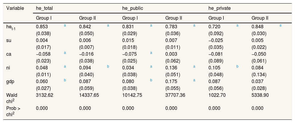
Sensitivity to alternative samples.
| Variable | he_total | he_public | he_private | |||||||||
|---|---|---|---|---|---|---|---|---|---|---|---|---|
| Group I | Group II | Group I | Group II | Group I | Group II | |||||||
| het-1 | 0.853 | a | 0.842 | a | 0.831 | a | 0.783 | a | 0.720 | a | 0.848 | a |
| (0.038) | (0.050) | (0.029) | (0.036) | (0.092) | (0.030) | |||||||
| su | 0.004 | 0.006 | 0.015 | 0.007 | −0.025 | 0.005 | ||||||
| (0.017) | (0.007) | (0.018) | (0.011) | (0.035) | (0.022) | |||||||
| ca | −0.058 | a | −0.016 | −0.075 | a | 0.003 | −0.081 | −0.050 | ||||
| (0.023) | (0.038) | (0.025) | (0.062) | (0.089) | (0.061) | |||||||
| ni | 0.048 | a | 0.094 | b | 0.034 | a | 0.136 | a | 0.105 | b | 0.084 | |
| (0.011) | (0.040) | (0.038) | (0.051) | (0.048) | (0.134) | |||||||
| gdp | 0.060 | b | 0.087 | 0.080 | b | 0.175 | a | 0.087 | 0.037 | |||
| (0.027) | (0.059) | (0.038) | (0.055) | (0.056) | (0.028) | |||||||
| Wald chi2 | 3132.62 | 14337.65 | 10142.75 | 37707.36 | 1022.70 | 5338.90 | ||||||
| Prob > chi2 | 0.000 | 0.000 | 0.000 | 0.000 | 0.000 | 0.000 | ||||||
Significant at 5%.
Standard errors are reported in brackets.
Number of observations: 361 and 190, for groups I and II, respectively. Group I: Australia, Austria, Belgium, Canada, Denmark, Finland, France, Germany, Iceland, Ireland, Italy, Japan, Luxembourg, Netherlands, Norway, Sweden, Switzerland, United Kingdom, and United States. Group II: Czech Republic, Greece, Hungary, Latvia, New Zealand, Poland, Portugal, Slovenia, Spain, and Turkey.
Firstly, per capita GDP has a positive effect on health. However, we show some differences when desegregating by health care financing schemes. It should also be noted that the ‘unit’ rule has limitations, especially, when elasticities of 0.01 and 0.99 are both classified as ‘necessities’. These numbers are economically and statistically quite different.
At this regard, higher elasticities are obtained for public health expenditures. Therefore, the smallest are for private ones. Overall, income elasticity is not as statistically significant when incorporating lags. That is, an anchorage effect is appreciated (0.80-0.90). In other words, about 80% of a year's health expenditure is conditioned by the previous one despite the presence of other explanatory variables.
Secondly, little effects are found for air quality variables as the most important factor again, and in accordance with previous evidence, appear to be income.23
As for air pollutants variables, the most important factor is the one regarding su in the linear estimations, whereas ca is for the dynamic one. These variables explain more private expenditures. A surprisingly fact here is the reverse effect of environmental factors here considered. For example, whereas su affect expenditures in a positive way in the linear one-way estimates, the reverse effect is obtained for the two-way. Neither stables results are obtained for ni. But regarding ca ones, stable negative effects are shown.
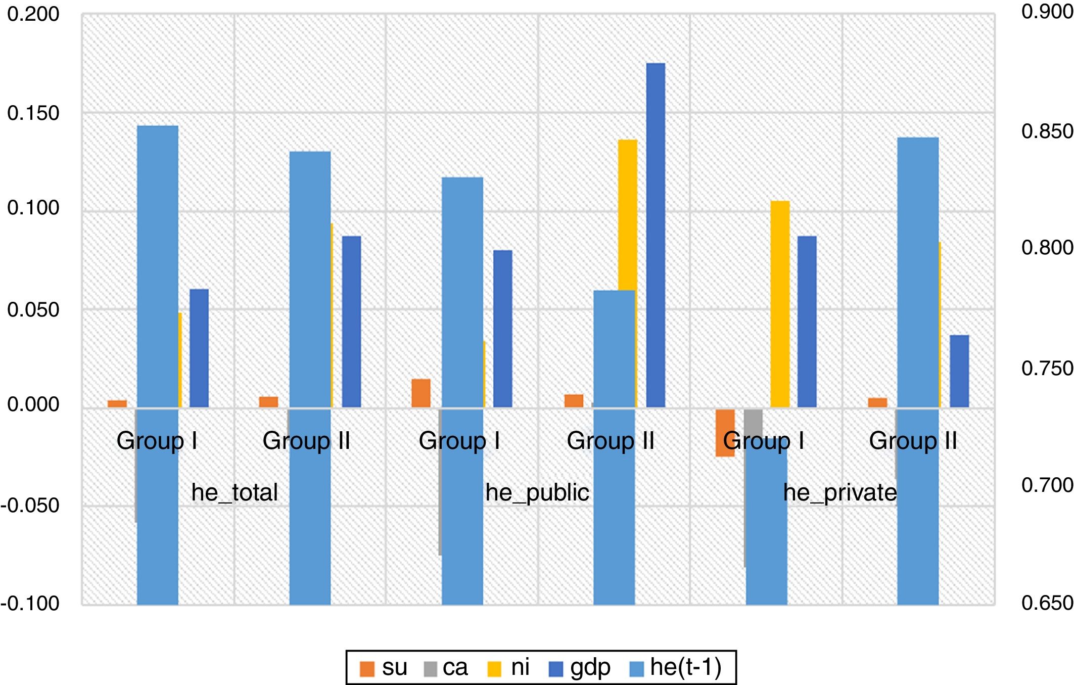
Robustness of resultsHere and now, we briefly test the robustness of the results. We noticed that the empirical model previously estimated imposes common effects for all the countries in the sample. To be more specific, Table 4 contains the results, while Figure 2 plots them.
Definitely, we check the sensitivity of the estimates to income heterogeneity in the sample of 29 OECD selected countries considered. In doing so, we split the sample of countries into two groups based on a kmeans and kmedians partition cluster analysis for income (considering 2005 base year, half of the period). Both methods are widely used for exploratory data analysis. Precisely, these partition methods break the observations into a distinct number of non-overlapping groups.
The first, group I, consist of 19 OECD countries: Australia, Austria, Belgium, Canada, Denmark, Finland, France, Germany, Iceland, Ireland, Italy, Japan, Luxembourg, Netherlands, Norway, Sweden, Switzerland, United Kingdom, and United States. While, 10 OECD countries constitute the second one, group II: Czech Republic, Greece, Hungary, Latvia, New Zealand, Poland, Portugal, Slovenia, Spain, and Turkey.
Specially, results highlighted the above-mentioned regarding the relevance of health expenditure in the previous period. Again, little differences are found by health care financing scheme.
When distinguishing by clusters, more statistically significant results are shown for group I. However, our findings are consisted between groups and when comparing with the full sample analysis. ni should be at main action agenda outlines, especially for group II, where higher elasticities are founded (i.e., 0.034 versus 0.136).
One of the implications of these interesting findings is that future health expenditure would increase as economic growth does, and the air quality indicators would do. Table IV in the online Appendix also tested how parameters for su, ni, and ca are different for countries with a lower or higher income by introducing interaction effects. DGDPi would be a dummy variable coded 1 for observations corresponding to countries in group I and 0 otherwise. Hence, general public policies, and especially those ones that contains health expenditure estimates, should contain reliable health care expenditure projections. That is, forecasts should take into account both traditional determinants (as income), including recent factors as population dynamics, population lifestyles or the technological progress; and other drivers, like the ones here analysed (air quality variables).24
DiscussionIn view of our outcomes, it may be concluded that we contribute to study the ecological and health economics literature regarding the impact of per capita income and environmental air quality variables on health expenditure determinants. Precisely, we try to solve the question regarding how air pollution could affect health care expenditures. Following recent literature, we studied the relationship between health expenditures and income (per capita), nitrogen, sulphur oxide, and carbon monoxide emissions. In doing so, we considered a balanced panel data of 29 selected OECD countries for the period 1995-2014. Besides, our main findings are also presented taking into account heterogeneity between countries.
In this spirit, our paper also provides a greater understanding of the underlying economic framework nested within the literature of health expenditure models.1,2 Our results are in accordance with previous contributions. Several measures here considered deteriorate air quality and so, negatively would affect health outcomes.3,5 However, it has been highlighted the importance of the economic conditions. Moreover, in our analysis nitrogen oxide emissions would have more significance than sulphur oxide emissions, or carbon monoxide ones that were considered in earlier studies.24,25
The cost savings of the health co-benefits achieved (health status, health care utilization and health expenditures)26,27 by policies to cut pollutants emissions are actually large.28,29 This is particularly important in the context here considered where health care expenditures are still growing. In any economic assessment of the costs of mitigation and adaptation, it should be considered the health bonus on savings. In spite of the vast evidence on health care expenditure determinants, there is still a need of further information. Science and public policy would benefit from additional research that integrates theory and practice from both air pollution effects to gain a better understanding of this issue.
Hence, in this study more empirical support is provided about how health management policies should include considerations for the use of cleaner fuels in the OECD countries. Overall, our results highlight that it is more crucial than ever to carry out an appropriate policy analysis at the macroeconomic level, which will allow policymakers to better allocate scarce resources. In an environment of financial constraints, every effort is short. Nonetheless, same health policies can have different effects, depending on the fiscal policy frameworks in which they are implemented.
All in all, it is important to highlight the research limitations and extensions of this study. But instead of dampening researchers’ spirits, limitations should serve to spur further research into an issue of vital importance. Limitations are mainly related to the OECD sample used (regions/countries, period and variables). In general, future research could include more environmental quality variables (more aspects than those associated to air pollution) related with health care expenditures (besides, more health outputs should be taken in mind) when considering all OECD countries or bearing in mind differences between developed and developing countries. When more data would be available, distinguishing by subperiods of time could be interesting, as for example, to consider other factors that lead to exhibit a significant association over the latest economic crisis. These and other issues could be considered as concerns of this interesting relationship that remains unexplained.
Editor in chargeCristina Linares Gil.
Transparency declarationThe corresponding author on behalf of the other authors guarantee the accuracy, transparency and honesty of the data and information contained in the study, that no relevant information has been omitted and that all discrepancies between authors have been adequately resolved and described.
Researchers are grappling with how best to characterize the effects of environmental air quality to address both health and environmental issues in a context of scarce resources. What is it well known is that air pollution is responsible for many adverse effects on health and well-being.
What does this study add to the literature?We use recently data and introduce new variables in estimates that make a new image of the traditional ones in order to provide support about how health management and policy makers should include new insights for the use of cleaner fuels.
All authors developed the idea and contributed to the concept and design. All authors contributed to the writing of the manuscript and read and approved the final manuscript.
A previous version of the paper was presented at the XXXVII Jornadas de Economía de la Salud organized by the Spanish Health Economics Association and the Spanish Epidemiological Society in Barcelona, 6 to 8 September 2017. We are grateful for the comments received for the participants.
Carla Blázquez-Fernández thanks Spanish Health Economics Association (AES) - Travel Expenses for attending XXXVII Jornadas AES (Barcelona).


