This paper aims the decomposition of the multidimensional Gini coefficient by deprivation to investigate how aggregate multidimensional poverty inequality translates into inequality within each of its components. This approach provides a better understanding of the distribution of deprivations held, the standard of living of the population and makes recommendations on government policies.
MethodWe use the method of Lerman and Yitzhaki (1985), which allows us to identify the impact of marginal changes on multidimensional inequality (fuzzy poverty inequality).
ResultsThe data used come from the Household Budget and Consumption Surveys of 2003 of 6695 households, 2011 of 9259 households and 2018 of 7493 households. Empirical findings suggest that the Gini index in 2003 is 0.229, 0.215 in 2011 and 0.180 in 2018.
ConclusionsThe different social policies to reduce multi-inequalities must mainly be oriented towards health policies and access to drinking water, which are unequally distributed during the three periods. And social policies to reduce inequality in education, sanitation and housing are also to be taken into account.
Este trabajo busca la descomposición del coeficiente de Gini multidimensional por privación para investigar cómo la desigualdad de pobreza multidimensional agregada se traduce en desigualdad dentro de cada uno de sus componentes. Este enfoque permite comprender mejor la distribución de las privaciones y el nivel de vida de la población, y formular recomendaciones sobre las políticas gubernamentales.
MétodoUtilizamos el método de Lerman y Yitzhaki (1985), que permite identificar el impacto de los cambios marginales sobre la desigualdad multidimensional (desigualdad difusa de la pobreza).
ResultadosLos datos utilizados provienen de las Encuestas de Presupuesto y Consumo de Hogares de 2003 en 6695 hogares, de 2011 en 9259 hogares y de 2018 en 7493 hogares. Los hallazgos empíricos sugieren que el índice de Gini en 2003 es 0,229, en 2011 es 0,215 y en 2018 es 0,180.
ConclusionesLas diferentes políticas sociales para reducir las desigualdades múltiples deben orientarse principalmente hacia las políticas de salud y acceso al agua potable, que se distribuyen de manera desigual durante los tres periodos. También deben tenerse en cuenta las políticas sociales para reducir la desigualdad en la educación, el saneamiento y la vivienda.
The continuous widening of inequalities in Africa is sometimes accompanied by an increase in poverty. The World Bank also recognizes that inequality can contribute decisively to poverty. Chad, like other African nations, has experienced high and increasing inequality over the years.
As part of policies to reduce poverty and inequality, the social health policy has contributed to improving health indicators: life expectancy of 48.06 in 2003 and 53.80 in 2018. Policies have been committed to ensuring food self-sufficiency, improving nutrition, increasing income and organizing markets. The energy, water and sanitation sectors have seen social actions. In the field of education, the targeted policies are the elimination of the gaps (girls/boys), training and employment.
Finally, specific actions to reduce gender inequalities and disparities have been carried out in favor of disadvantaged groups (women and men).
However, in Chad, social policies for poverty and inequality reduction seem to result in a decline in income poverty: 54.8% in 2003, 46.7% in 20111 and 42.3% in 2018, but they are often not sufficient to significantly modify the structure of income distribution (according to World Bank, Gini index: 0.398 in 2003, 0.433 in 2011 and 0.375 in 2018). They must now direct resources towards the underprivileged and target groups at risk. This involves analyzing the multi-inequality of different subgroups of households on the basis of certain criteria, such as place of residence and sex of the head of household. The construction of a profile of poverty inequality facilitates the formulation of targeted measures in the context of the fight against poverty and inequality.
Earlier empirical works on income inequality have tried to decompose using the additive decomposition method of Rao.2–4 Unlike previous approaches, Shorrocks5,6 also proposed a method to decompose inequality, as measured by the squared coefficient of variation.
In 1985, Lerman and Yitzhaki7 developed and used a new method to decompose income inequality by factor components in the US (1980). This approach is used in many countries.8–15
Chakravarty16 introduced a method that can be simultaneously decomposed into subgroups and attributes.
The authors17–19 used the method of Dagum20,21 to decompose Gini income inequality.
We use for the decomposition the Gini index proposed by Lerman and Yitzhaki, which allows us to identify the impact of marginal changes on inequality.
MethodDataThe data sources come from harmonized surveys on household living conditions, an initiative of the West Africa Economic Monetary Union (WAEMU) Commission. They are carried out by the National Statistical Institutes (INSEED). Samples of households surveyed: 7493 households in 2018, 9259 in 2011 and 6695 in 2003.
The samples are representative at the national level with stratifications by area of residence (urban/rural) and region. The sampling unit is the ordinary household residing in the field of the survey.
The sampling frames are made up of the exhaustive list of the 6,685 and 12,150 enumeration areas (ZD) taken from the first and second Population and Housing Censuses (RGPH1 [1993]; RGPH2 [2009]). Enumeration areas are distinct, nonempty area units that cover the entire country. They form a partition of the national territory and are constituted in such a way that each contains approximately a thousand inhabitants. A ZD contains an average of 200 households.
These surveys were carried out on the basis of a two-stage area sample with first-stage stratification; ZD was the primary survey unit (584 ZDs in 2003, 850 in 2011 and 625 in 2018). Each region is divided into two strata: urban and rural. Given the specificity of the city of N’Djamena, each of its 10 districts constitutes an urban stratum. At the second level, we proceeded to a systematic selection of households after having carried out an exhaustive enumeration of households in the sample ZD (12 households per ZD in 2003, 2011 and 2018).
The number of households in Chad is estimated to be 1,258,710 in 2003, 1,784,040 in 2011 and 2,931,672 in 2018.
Choice and description of variablesThe question of the choice of deprivation indicators has been discussed at length by Cheli et al.22 and by Cheli and Lemmi23. These authors note that the choice of deprivation indicators is of fundamental importance. Furthermore, they recommend, in the analysis, clearly distinguishing the effect variables and the cause variables from poverty.
Finally, Miceli24 points out that the choice of deprivation indicators is particularly delicate and cannot intervene without a dose of arbitrary more or less and that the fuzzy measurement obtained is ultimately conditioned by the data availability.
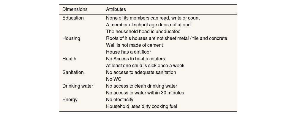
The deprivation thresholds first identify the people experiencing deprivation in each selected indicator. Attribute deprivation is dichotomous and component of dimension. Dimensional deprivation is defined by the total deprivation of its attributes. Table 1 details the variables (dimensions and attributes) used in this paper.
List of dimensions and attributes.
| Dimensions | Attributes |
|---|---|
| Education | None of its members can read, write or count |
| A member of school age does not attend | |
| The household head is uneducated | |
| Housing | Roofs of his houses are not sheet metal / tile and concrete |
| Wall is not made of cement | |
| House has a dirt floor | |
| Health | No Access to health centers |
| At least one child is sick once a week | |
| Sanitation | No access to adequate sanitation |
| No WC | |
| Drinking water | No access to clean drinking water |
| No access to water within 30 minutes | |
| Energy | No electricity |
| Household uses dirty cooking fuel |
Note: variables selected by the author.
Fuzzy indices of poverty (multidimensional poverty) provide a framework for better understanding poverty through its multiple facets.
Consider a population P of n households and the attribute Xjj=1,…,m:
and fai is the weight of household ai in the sample by imposing xij=1, if the household ai does not have the attribute j, else xij=0.And f(ai)/∑i=1nf(ai) is the relative frequency represented by the sample observation ai in the total population.
The weight of household ai in the sample (extrapolation or dilation coefficient) is defined by:
and fai is the inverse of the probability for any household ai to belong to the sample in the county.M is the total number of ZDs in the county; m is the total number of ZDs in the sample (primary units) in county; ni is the number of households ai sampled (secondary units) for the survey in the ZD in the sample; and Ki is the number of households obtained during the enumeration of the ZD of the household ai.
ZDs were drawn without replacement with equal probability as well as second-degree households.
The ratio μXj reflects the degree of deprivation of attribute Xj for the population of n households.
Dagum and Costa25 introduced decomposition by attribute by demonstrating that it is possible to calculate the contribution of attribute Xj to the overall fuzzy poverty index.
The fuzzy poverty index is defined as:
with wj=Log∑i=1nf(ai)/∑i=1nf(ai)26. wj is the weight attached to the attribute Xj=x1j, x2j,…, xij,…, xnj.The authors obtain the (absolute) contribution of attribute Xj to the multidimensional poverty index:
where μj=μXjwj/∑j=1mwj.We adopt the Gini decomposition method introduced by Lerman and Yitzhaki. The Gini coefficient is treated as an indicator of inequality in the distribution of the fuzzy poverty ratio in the population, and the formula is given as the covariance of the fuzzy poverty index (μ), the cumulative distribution of μ: F and the mean of the fuzzy poverty index (μ) in p of n households:μ¯= ∑i=1nμaifai/∑i=1nfaiwithη(ai)=∑j=1mxijwj/∑j=1mwj27.
The Gini coefficient is defined by:
Then, following Lerman and Yitzhaki, the fuzzy poverty index is decomposed such that:
The components are education, housing, health, sanitation, drinking water and energy.
Fj represents the cumulative distribution of μj, and μ¯j is the mean. Therefore, the Gini coefficient of the jth component is calculated as:
As η=∑j=1mηj, we have η¯j=∑i=1nηj(ai)f(ai)/∑i=1nf(ai)with μjai=xijwj/∑j=1mwj (see equations 1, 3 and 4).
Then, utilizing the cumulative distributions and averages of the fuzzy poverty ratio. The Gini coefficient of the fuzzy poverty index would be expressed as:
Based on Lerman and Yitzhaki, we combine the equations above and show that the relative Gini coefficient can be decomposed as follows:
Thus:
where Rj is the correlation between the contribution of attribute Xj and the fuzzy poverty index, Gj is the Gini coefficient for each of the fuzzy poverty index components and Sj is the contribution to the fuzzy poverty index of the jth component.Equation 9 indicates that any change in the variables Rj,Gj or Sj will be mirrored by changes in Cj. The higher the value of one of these components, the more Cj increases, and the more the fuzzy poverty index inequality increases since G=∑j=1mCj.
A primary reason for using this decomposition approach is its usefulness in examining how marginal changes to the fuzzy poverty index for particular components can affect overall inequality.
If a fuzzy poverty index source represents a large share of total inequality, it may potentially have a large impact on inequality. However, if the fuzzy poverty index is equally distributed (G=0), it cannot influence inequality, even if its magnitude is large. On the other hand, if this fuzzy poverty index source is large and unequally distributed (Sj and Gj are large), it may either increase or decrease inequality, depending on which households (individuals), at which points in the fuzzy poverty index distribution, earn it. If the fuzzy poverty index source is unequally distributed and flows disproportionately toward those at the top of the fuzzy poverty index distribution (Rj is positive and large), its contribution to inequality will be positive.
We also measure the relative efects of inequality by calculating both the relative fuzzy poverty index inequality (Ij=CjG) and the relative marginal effects (Ij−Sj).
The Gini coefficients are popular measures of inequality. Similarly, concentration coefficients (Concj=Gj*Rj) are often used to measure income-related inequalities in other socially important variables.
The decomposition method discussed above allows for the estimation of bootstrapped standard errors and confidence intervals to ascertain the robustness of the results.
We use the command, sgini in stata, which decomposes the Gini coefficient by a fuzzy poverty index source and allows the calculation of the impact that a marginal change in a particular fuzzy poverty source will have on inequality.7,28
Empirical resultsAnalysis of fuzzy povertyIn Table 2, the weight wj represents the intensity of deprivation linked to the attribute Xj. The weights of Cerioli and Zani26 are defined according to an inverse relation of the average degree of deprivation relative to the indicator j. According to this weighting system, more weight is assigned to the most common indicators.
Fuzzy poverty index in 2003, 2011 and 2018.
| 2003 | 2011 | 2018 | ||||||||||
|---|---|---|---|---|---|---|---|---|---|---|---|---|
| Dimensions | wj | μj | μj | μjμ | wj | μj | μj | μjμ | wj | μj | μj | μjμ |
| Education | 0.173 | 0.638 | 0.110 | 0.226 | 0.266 | 0.643 | 0.171 | 0.290 | 0.270 | 0.649 | 0.175 | 0.273 |
| Housing | 0.108 | 0.808 | 0.088 | 0.180 | 0.101 | 0.833 | 0.084 | 0.143 | 0.196 | 0.708 | 0.139 | 0.217 |
| Health | 0.317 | 0.389 | 0.123 | 0.253 | 0.319 | 0.445 | 0.142 | 0.240 | 0.204 | 0.600 | 0.123 | 0.192 |
| Sanitation | 0.076 | 0.727 | 0.055 | 0.113 | 0.076 | 0.742 | 0.056 | 0.096 | 0.024 | 0.924 | 0.022 | 0.034 |
| Drinking water | 0.317 | 0.322 | 0.102 | 0.209 | 0.233 | 0.558 | 0.130 | 0.221 | 0.270 | 0.558 | 0.151 | 0.235 |
| Energy | 0.010 | 0.972 | 0.010 | 0.021 | 0.006 | 0.986 | 0.006 | 0.010 | 0.035 | 0.928 | 0.032 | 0.050 |
| Chad | 1.000 | 0.487 | 0.487 | 1.000 | 1.000 | 0.589 | 0.589 | 1.000 | 1.000 | 0.642 | 0.642 | 1.000 |
Note: author's calculations, μ=∑j=16μj and μj=wj*μj.
The fuzzy poverty indices in Chad are 0.487 in 2003, 0.589 in 2011 and 0.642 in 2018. In other words, Chadian households were 48.7% structurally poor in 2003, 58.9% in 2011 and 64.2% in 2018, while the monetary poverty stood at 54.8% in 2003, 46.7% in 2011 and 42.3% in 2018.
According to the decomposition by attribute developed by Dagum and Costa,25 the indices of the dimensions of poverty that have important parts in the construction of the one-dimensional fuzzy index of poverty in 2003 are μ(education) = 0.638; μ(housing) = 0.808; μhealth=0.389; μ(sanitation) = 0.727; and μdrinking water=0.322μ(energy) = 0.972. in 2011, we have μ(education) = 0.643, μ(housing) = 0.833, health=0.445; μ(sanitation) = 0.742; μdrinking water=0.558; μ(energy) = 0.986. And in 2018, we have μ(education) = 0.649, μ(housing) = 0.708, μhealth=0.445; μ(sanitation) = 0.924; μdrinking water=0.558; μ(energy) = 0.928.
The decrease in the relative contribution of health to multidimensional poverty during these three periods would be justified by the importance that Chad gives to health policy.
Gini index decomposition in multidimensional povertyThe Gini coefficient is a ratio between 0 and 1 that measures the distribution of inequality. The rate of inequality increases as it gets closer to 1 and decreases as it gets closer to zero. It is treated as an indicator of inequality in the distribution of the fuzzy poverty ratio in the population.
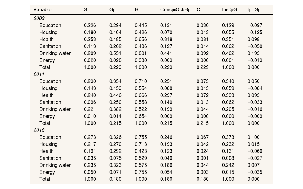
Table 3 gives the overall Gini coefficients in the fuzzy poverty index at 0.229 in 2003, 0.215 in 2011 and 0.180 in 2018.
Inequality effects by deprivation.
| Variable | Sj | Gj | Rj | Concj=Gj∗Rj | Cj | Ij=Cj/G | Ij− Sj |
|---|---|---|---|---|---|---|---|
| 2003 | |||||||
| Education | 0.226 | 0.294 | 0.445 | 0.131 | 0.030 | 0.129 | −0.097 |
| Housing | 0.180 | 0.164 | 0.426 | 0.070 | 0.013 | 0.055 | −0.125 |
| Health | 0.253 | 0.485 | 0.656 | 0.318 | 0.081 | 0.351 | 0.098 |
| Sanitation | 0.113 | 0.262 | 0.486 | 0.127 | 0.014 | 0.062 | −0.050 |
| Drinking water | 0.209 | 0.551 | 0.801 | 0.441 | 0.092 | 0.402 | 0.193 |
| Energy | 0.020 | 0.028 | 0.330 | 0.009 | 0.000 | 0.001 | −0.019 |
| Total | 1.000 | 0.229 | 1.000 | 0.229 | 0.229 | 1.000 | 0.000 |
| 2011 | |||||||
| Education | 0.290 | 0.354 | 0.710 | 0.251 | 0.073 | 0.340 | 0.050 |
| Housing | 0.143 | 0.159 | 0.554 | 0.088 | 0.013 | 0.059 | −0.084 |
| Health | 0.240 | 0.446 | 0.666 | 0.297 | 0.072 | 0.333 | 0.093 |
| Sanitation | 0.096 | 0.250 | 0.558 | 0.140 | 0.013 | 0.062 | −0.033 |
| Drinking water | 0.221 | 0.382 | 0.522 | 0.199 | 0.044 | 0.205 | −0.016 |
| Energy | 0.010 | 0.014 | 0.654 | 0.009 | 0.000 | 0.000 | −0.009 |
| Total | 1.000 | 0.215 | 1.000 | 0.215 | 0.215 | 1.000 | 0.000 |
| 2018 | |||||||
| Education | 0.273 | 0.326 | 0.755 | 0.246 | 0.067 | 0.373 | 0.100 |
| Housing | 0.217 | 0.270 | 0.713 | 0.193 | 0.042 | 0.232 | 0.015 |
| Health | 0.191 | 0.292 | 0.423 | 0.123 | 0.024 | 0.131 | −0.060 |
| Sanitation | 0.035 | 0.075 | 0.529 | 0.040 | 0.001 | 0.008 | −0.027 |
| Drinking water | 0.235 | 0.323 | 0.575 | 0.186 | 0.044 | 0.242 | 0.007 |
| Energy | 0.050 | 0.071 | 0.755 | 0.054 | 0.003 | 0.015 | −0.035 |
| Total | 1.000 | 0.180 | 1.000 | 0.180 | 0.180 | 1.000 | 0.000 |
Note: author's calculations.
In 2003, the increase in Gini coefficients in fuzzy poverty is attributed to drinking water (0.0922) and health (0.081), in 2011, education (0.073), health (0.072) and drinking water (0.044) and in 2018, education (0.067), drinking water (0.044) and housing (0.042).
The main sources of absolute contribution to inequality in 2003 were drinking water (0.092), health (0.0805) and education (0.030) in 2003, education 0.073), health (0.072) and drinking water (0.044) in 2011 and education (0.067), drinking water (0.044) and housing (0.042) in 2018.
The fuzzy share (Sj) and Share Inequality (Ij) sources of fuzzy poverty indices that have large shares of total inequality have a potentially large impact on inequality. In 2003, health and drinking water have a potentially large impact on the inequality, in 2011, we have education, health and drinking water and in 2018, the education, housing and drinking water.
The high concentration coefficients and the correlation with the rank of inequality also contribute to the increase in inequality.
A positive marginal effect coefficient indicates that an increase in the fuzzy poverty ratio for the component will increase inequality: in 2003, health and drinking water, in 2011, education and health and in 2018, education, housing and drinking water.
During the three periods, the Gini coefficients experienced successive declines for health, sanitation and drinking water.
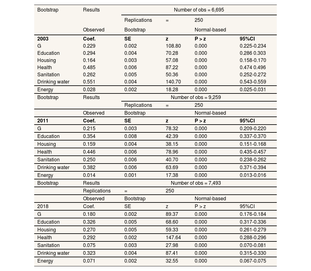
Bootstrap resultsThe simple bootstrap allows assigning measures of accuracy such as Gini coefficient, variance, and confidence intervals to the sample estimates.29 In Table 4, column 1 shows the fuzzy poverty index components, respectively, and column 5 gives the confidence interval and shows that they are all significant.
Bootstrap results in 2003, 2011 and 2018.
| Bootstrap | Results | Number of obs = 6,695 | |||
|---|---|---|---|---|---|
| Replications | = | 250 | |||
| Observed | Bootstrap | Normal-based | |||
| 2003 | Coef. | SE | z | P > z | 95%CI |
| G | 0.229 | 0.002 | 108.80 | 0.000 | 0.225-0.234 |
| Education | 0.294 | 0.004 | 70.28 | 0.000 | 0.286 0.303 |
| Housing | 0.164 | 0.003 | 57.08 | 0.000 | 0.158-0.170 |
| Health | 0.485 | 0.006 | 87.22 | 0.000 | 0.474 0.496 |
| Sanitation | 0.262 | 0.005 | 50.36 | 0.000 | 0.252-0.272 |
| Drinking water | 0.551 | 0.004 | 140.70 | 0.000 | 0.543-0.559 |
| Energy | 0.028 | 0.002 | 18.28 | 0.000 | 0.025-0.031 |
| Bootstrap | Results | Number of obs = 9,259 | |||
| Replications | = | 250 | |||
| Observed | Bootstrap | Normal-based | |||
| 2011 | Coef. | SE | z | P > z | 95%CI |
| G | 0.215 | 0.003 | 78.32 | 0.000 | 0.209-0.220 |
| Education | 0.354 | 0.008 | 42.39 | 0.000 | 0.337-0.370 |
| Housing | 0.159 | 0.004 | 38.15 | 0.000 | 0.151-0.168 |
| Health | 0.446 | 0.006 | 78.96 | 0.000 | 0.435-0.457 |
| Sanitation | 0.250 | 0.006 | 40.70 | 0.000 | 0.238-0.262 |
| Drinking water | 0.382 | 0.006 | 63.69 | 0.000 | 0.371-0.394 |
| Energy | 0.014 | 0.001 | 17.38 | 0.000 | 0.013-0.016 |
| Bootstrap | Results | Number of obs = 7,493 | |||
| Replications | = | 250 | |||
| Observed | Bootstrap | Normal-based | |||
| 2018 | Coef. | SE | z | P > z | 95%CI |
| G | 0.180 | 0.002 | 89.37 | 0.000 | 0.176-0.184 |
| Education | 0.326 | 0.005 | 68.60 | 0.000 | 0.317-0.336 |
| Housing | 0.270 | 0.005 | 59.33 | 0.000 | 0.261-0.279 |
| Health | 0.292 | 0.002 | 147.64 | 0.000 | 0.288-0.296 |
| Sanitation | 0.075 | 0.003 | 27.98 | 0.000 | 0.070-0.081 |
| Drinking water | 0.323 | 0.004 | 87.41 | 0.000 | 0.315-0.330 |
| Energy | 0.071 | 0.002 | 32.55 | 0.000 | 0.067-0.075 |
95%CI: 95% confidence interval; SE: standard error.
Note: author's calculations.
The series of data presented in this paper is key to understanding the evolution of fuzzy poverty index inequality in Chad in 2003, 2011 and 2018.
According to World Bank data, income inequality was 0.398 in 2003, 0.433 in 2011 and 0.375 in 2018 in Chad, while inequality in fuzzy poverty was 0.229 in 2003, 0.215 in 2011 and 0.180 in 2018.
The Chad's 2018 Gini index dropped sharply to 0.375 (World Bank) and the Gini index in the multidimensional poverty drop to 0.180. The result of our study confirms this decrease. The results in this study show that a 1% increase in this source of the fuzzy poverty index, all else being equal, increases the Gini coefficient of the fuzzy poverty index by 0.098 for health and 0.193 for drinking water in 2003, 0.050 for education and 0.093 for health in 2011 and 0.100 for education, 0.015 for housing and 0.007 for drinking water in 2018.
In Chad, health and drinking water are not evenly distributed (0.485 for health and 0.551 for drinking water), and the Gini correlations between their fuzzy poverty ratios and the fuzzy poverty index (0.656 for health and 0.801 for drinking water) in 2003 indicate that deprivation in health and drinking water affects the disadvantaged more than other sources of deprivation. In 2011, health (0.446) and education (0.354) also show unequal distributions with strong correlations with the rank of inequality. In 2018, education (0.326), housing (0.270), drinking water (0.323) and health (0.292) are unequal distributions with strong correlations with the rank of inequality.30
Using the income distribution or consumption expenditure distribution, work was subsequently carried out on inequalities, Shorrocks5,6 propose rules for decomposing measures of income inequality either by subgroup (subpopulation) or by source of income.
The concept of multi-decomposition is well suited to propose new measures of changes in inequality in a context where policy simulations are analyzed using the fuzzy poverty index. The application of these analytical tools can provide rich and useful information in the context of policy impact analysis. These may shed more light on various reforms and help in the design of inequality-reducing tax reforms as well as compensatory targeting policies, which are valuable elements in the implementation process of policy reforms, Mussard and Pi Alperin in Argentina18 and Mussard and Savard in Phillipines.19 Unlike the decomposition of monetary inequality using either the distribution of income or consumption expenditure, this method allows us to have the various non-monetary inequalities: education, housing, health, sanitation, drinking water and energy. These indices constitute complementary instruments for the fight against poverty and inequality, including the non-monetary dimensions that escape current instruments. The limits of the reduction of inequality would find its justification in the absence of taking into account the non-monetary dimensions of inequality.
A fuzzy approach is quite appropriate if there are quantitative variables involved in the analysis along with categorical and dichotomous variables. However this is not the case in this paper. The selected variables are the dichotomous variables and the lack of the income dimension would be justified by the fact that it would already act on almost all the other dimensions selected (for example having a permanent home depends on its income, energy, etc.). Finally, Miceli24 points out that the choice of deprivation indicators is particularly delicate and cannot intervene without a dose of arbitrary more or less and that, the fuzzy measurement obtained is ultimately conditioned by the data availability. The selection of socio-economic attributes to study the state of poverty was made on the basis of multidimensional notions of poverty, information from the Ecosit4 (2018), Ecosit3 (2011) and Ecosit2 (2003) surveys and the Sustainable Development Goals.
Finally, further research is needed to resolve both fuzzy poverty index disparities across population subgroups, as well as regional disparities in fuzzy poverty. Such subgroup research would facilitate the investigation of changes in the distribution of consumption expenditures over time, as well as the examination of possible factors leading to either the increase or decrease in inequality.
The paper aims the different social policies to reduce multi-inequalities must mainly be oriented towards health policies and access to drinking water, which are unequally distributed during the three periods. And social policies to reduce inequality in education, sanitation and housing are also to be taken into account.
Several studies have been done on monetary poverty, multidimensional poverty and monetary inequality to fight poverty and inequality.
What does this study add to the literature?The multi-inequality calculated from the fuzzy index of poverty (multidimensional poverty) makes it possible to know the non-monetary sources of multidimensional poverty. Few studies have used the fuzzy poverty index to calculate multi-inequality.
What are the implications of the results?Knowledge of these sources of fuzzy inequality allows the government and other political decision-makers to orient their policy of the fight against inequality towards these sources of deprivation.
Carlos Álvarez-Dardet.
Authorship contributionsThe data comes from the Institute of Statistics of Chad (INSEED); the statistical analysis and interpretations of the data are my responsibility.
FundingNone.
Conflicts of interestNone.


